Portfolio Project Report
Note: Code for this project can be found on my GitHub.
Data Set Summary & Exploration
1. Basic summary of the data set.
In order to calculate summary statistics for the data set, I used numpy library. The results are as follows:
- The size of training set is 34799 images.
- The size of the validation set is 4410 images.
- The size of test set is 12630 images.
- The shape of a traffic sign image is 32x32x3. This means that each picture is 32 pixels wide, 32 pixels tall, and has 3 color channels.
- The number of unique classes/labels in the data set is 43.
2. Exploratory visualization of the dataset.
First of all, I decided to plot some random traffic signs from the train data set. To do that, I generated random indices, retreived 25 corresponding images and then plotted them. Visualization can be seen below. The first thing that caught my attention was that lighting conditions under which the photos were taken can vary quite drastically. Some of the photos are really hard to tell apart because the lighting was so dark. I consider this can be a challenge for a neural network.
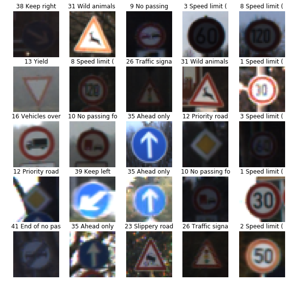
Random sample of 25 road signs.
Another part that is really important for any classification task is the possible problem of class imbalance. In order to see whether this problem exists for this task, I decided to plot a simple histogram showing the number of training examples for each class. The result can be seen below.
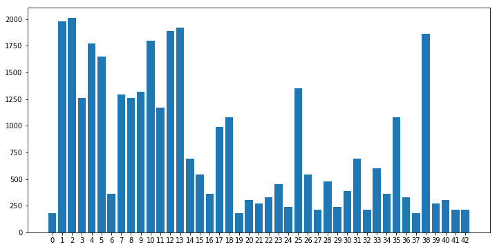
HIstogram of the 43 classes of traffic signs. Note that classes are imbalanced.
It is clear that there are quite unbalanced classes in the data set. This means that the model might learn well good represented classes and might not learn well under-represented classes. In order to solve this issue, I balanced the classes in such a way that all of them have equal number of images.
Design and Test a Model Architecture
1. Image preprocessing.
The first step that I took in data preprocessing was normalizing all the pictures by substracting mean value and dividing by the standard deviation of the mean value. This normalization was performed for each of 3 of the color channels. This approach was inspired by the famous VGG19 paper that won prestigious ImageNet competition in 2014. I normalized all train, validation and test data sets using this approach. An important consideration was data leakage, so the mean and SD values used for all normalization were calculated only based on the training data set, and not validation or test data.
The next two steps were class balancing and data augmentation using 3 types of transformation: rotation, translation and shear. I used CV2 package to do this. I decided that combining these two steps together makes sense, because simply copying images in under-represented classes might make the network memorize data instead of learning important internal representation of features. I played with different values of transformation parameters until I was satisfied with results. Resulting transformed images can be seen below.
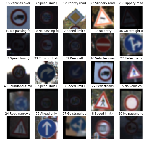
Random sample of 25 augmented traffic signs. I used rotation, translation and shear to increased variability of data during training.
After augmentation/balancing, each class has 2010 images, which is how many images the largest class had before augmentation. Histogram of post-augmentation class distribution follows below (it is quite boring in fact, due to all classes having same number of examples).
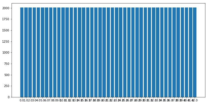
Histogram of dataset after random resampling with replacement was performed to make all classes equally represented.
2. Model architecture.
My final model consisted of the following layers:
| Layer | Description |
|---|---|
| Input | 32x32x3 RGB image |
| Convolution 1x1 | 1x1 stride, 3 kernels, valid padding, outputs 32x32x3 |
| Convolution 3x3 | 1x1 stride, 16 kernels, valid padding, outputs 30x30x16 |
| RELU | |
| Dropout | pkeep = 0.65 |
| Convolution 3x3 | 1x1 stride, 32 kernels, valid padding, outputs 28x28x32 |
| RELU | |
| Dropout | pkeep = 0.65 |
| Max Pool | 2x2 stride, 2x2 kernel size, outputs 14x14x32 |
| Convolution 3x3 | 1x1 stride, 64 kernels, valid padding, outputs 12x12x64 |
| RELU | |
| Dropout | pkeep = 0.65 |
| Max Pool | 2x2 stride, 2x2 kernel size, outputs 6x6x64 |
| Flatten | Outputs 2304 |
| Dense Layer | 256 neurons, outputs 256 |
| RELU | |
| Dropout | pkeep = 0.65 |
| Dense Layer | 128 neurons, outputs 128 |
| RELU | |
| Dropout | pkeep = 0.65 |
| Output Layer | 43 neurons, outputs 43 |
| Softmax | Outputs 43 logits |
This architecture was originally inspired by the famous LeNet, but then modified during trial-and-error and also studying other architectures.
The first layer is quite interesting, in my opinion. It has 3 1x1 convolution channels. What this allows to do is for the network to learn “the best” color channel combination. I originally saw this in VGG19 paper, but then read online that many people use it. It turns out that original RGB color scheme sometimes is not the best for deep learning and we can make a network learn for itself what the most efficient combination of RGB channels. This can improve accuracy.
Another point of attention should be max pooling layers. The first convolutional layer (1x1 doesn’t count) doesn’t have max pooling, whereas the other two do have 2x2 max pooling. You may ask why, and the answer has to do with dimesionality reduction. Had I used max pooling after first layer, the output from which has 30x30 spacial dimansion, and after max pooling that would be 15x15, which after next convolutional layer would be 13x13, at which point 2x2 max pooling cannot be applied. This means I needed to plan convolutional and max pooling layers in such a fashion that all corresponding input-output spacial dimensions are even number of pixels.
Apart from these 2 points, I do not think that anything else stands out about this architecture.
3. Training the model.
To train the model, I made the following decisions:
- Adam optimizer. Adam optimizer uses adaptive decrease of the learning rate. It is quite useful, as it allows the optimizing algorithm to slow down as it approaches solution.
- Starting learning rate of 0.0005. This choice was motivated by trial and error and also by looking at what practitioners use for this type of optimizer.
- Batch size of 32. I was getting out of memory errors when trying to make this value larger, so I decided to stop at 32.
- Number of epochs was 201. Since one epoch trained relatively fast (14 seconds on average), I could afford to run it for longer and see if it converges to some value (which it did).
4. Finding the final solution.
In the graph below, the blue line represents training accuracy and the orange line represents validation accuracy. In the beginning of the training, validation accuracy is higher than training accuracy. This is the result of using dropout. This reduces training accuracy and prevents overfitting. Using dropout additionally reduces the gap between training and validation accuracy, which is good. On the downside, training requires more epochs to converge.
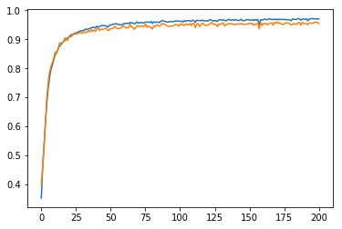
Vertical axis: accuracy; horizontal axis: number of training epochs. Blue line: train accuracy; orange line: test accuracy.
After training the model for 201 epochs, the final results were:
- training set accuracy of 0.971
- validation set accuracy of 0.954
- test set accuracy of 0.9376
During this project, I have tried many architectures and encountered numerous challenges. Unfortunately, I did not keep a log of all approaches that I tried.
I started out with the LeNet architecture. Originally, I was choosing between LeNet and VGG16. I went with LeNet because VGG16 is used for a much more complex images including hundreds and thousands of classes and I thought it would be an overkill. In addition, transfer learning even for VGG16 can take quite some time and I did not have access to a very good GPU at that point in time. So LeNet was my choice because it was a simple architecture and training time would be shorter. Also I chose it because, in my opinion, both MNIST digits data set (originally used for LeNet) and traffic signs are similar in complexity in the sense that both are have very simple fatures that distinguish classes (as compared with distinguishing cats from dogs, which is much harder).
The LeNet did not work well for me. I started doing some reading about convnet architectures, and also had a look at what other students did for this project to get some inspiration.
I read about VGG19 that mentions 1x1 convolutions in the first layers and also saw other people use it, so I decided to give it a go. Then I also decided to increase complexity of the model and increased number of kernels in the first 3 convolutional layers to be 16-32-64.
This led to overfitting. Training accuracy was quickly going to 1.0, which means the network was simply “memorizing” the data and not learning. At the same time validation accuracy was stuck at around 88%, which is not enough.
I needed to regularize. I watched this amazing Tensorflow tutorial by Martin Görner. After that I knew that dropout was a good way to regularize. 0.5 dropout was too much, the model was not learning (or maybe it was, just way too slow), I reduced dropout to 0.35 (pkeep of 0.65) and got very good result, which still was below 0.93 needed for this project.
I played quite a bit with different parameters, witch very little effect until I decided to increase the number of neurons in fully connected layers tp 256 and 128, accourdingly. This is when my validation performance finally went over 93%, at which point I was really excited, especially after frustration times, when nothing really worked.
Finally, training, validation and test accuracy are all realtively close to each other, and all are higher than 0.93. This means that my model is working and can be expected to perform better than 93% on a relatively large data set of unseen images.
Test a Model on New Images
1. New German traffic signs.
Here are six German traffic signs that I found on the web:
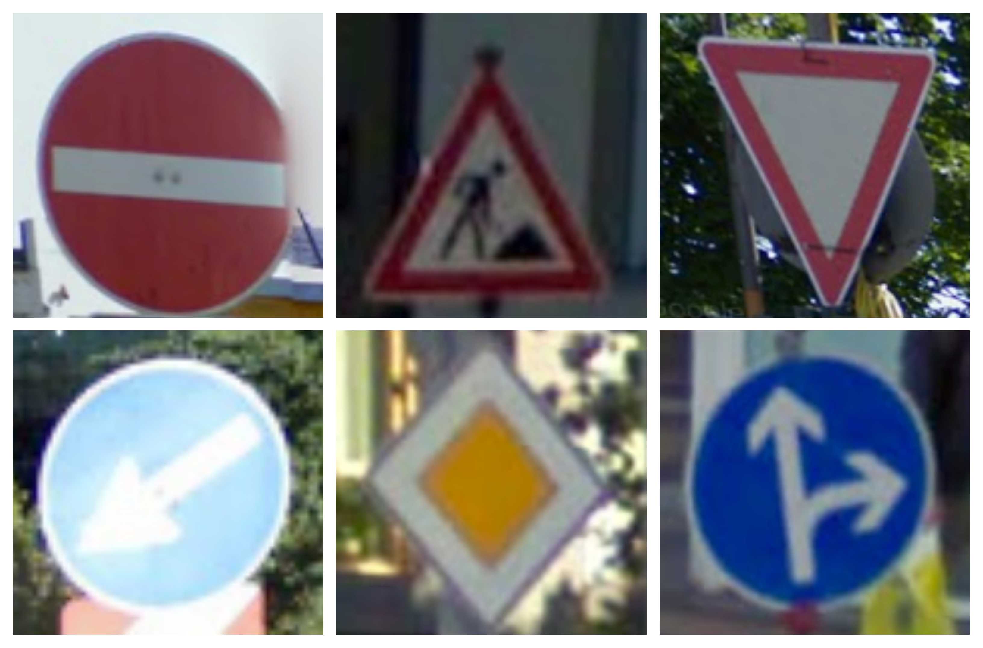
Six German signs clipped from Google maps street view for testing the model.
I cut them manually from Google maps, this is why they are all different sizes. When using them for predictions, I used CV2 to resize them to 32x32 pixels. It was not easy to find the signs. I entered street view on a random street in Berlin and spend around an hour collecting signs. I think I was not lucky and that area did not have too many signs.
All the signs photos look like they should not be a challenge for the model to classify. None of them were taken in low light conditions. Neither do they have significant distortions.
2. Model’s predictions on the new traffic signs.
Here are the results of the prediction:
| Image | Prediction | Correct? |
|---|---|---|
| No entry | No entry | Yes |
| Road work | Road work | Yes |
| Yield | Yield | Yes |
| Keep left | Go straight of left | No |
| Priority road | Priority road | Yes |
| Go straight or right | Go straight or right | Yes |
| Accuracy | 0.8333 |
Accuracy of predictions for new images was 0.8333. This is lower than the accuracy for the test set of 0.937. Explanation is quite simple, the set of new images is too small and one error makes overall accuracy much lower than test set accuracy. For a more valid assessment, in my opinion, a larger set of new images is needed.
3. Softmax probabilities for all new signs.
The code for making predictions on my final model is located in the 62th cell of the Ipython notebook.
Results can be seen in the figure below.
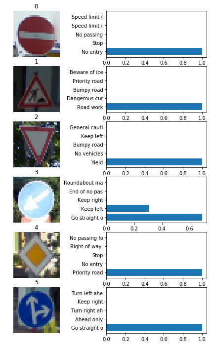
Caption
For 5 out of 6 images, the model is extremely confident in what it thinks the class of an image is. For all of those images, the predictions are correct. This is why I will not provide tables with probabilities for all the correct images. Precise numbers can be seen in the notebook after cell 74.
The only image for which the model is not confident, turns out to be the image where the model made a mistake. The model predicted it to be class 37 with probability of 68.9% (incorrect) and the second prediction 30.99% was for the correct class 39. By examining the photo we can see that the sign is too bright and this might have confused the model.
| Probability | Prediction |
|---|---|
| 0.6890 | [Class 37] Go Straight or Left |
| 0.3099 | [Class 39] Keep Left |