Part of Understanding Hinton’s Capsule Networks Series:
- Part 1: Intuition
- Part 2: How Capsules Work
- Part 3: Dynamic Routing Between Capsules (you are reading it now)
- Part 4: CapsNet Architecture
Introduction
This is the third post in the series about a new type of neural network, based on capsules, called CapsNet. I already talked about the intuition behind it, as well as what is a capsule and how it works. In this post, I will talk about the novel dynamic routing algorithm that allows to train capsule networks.
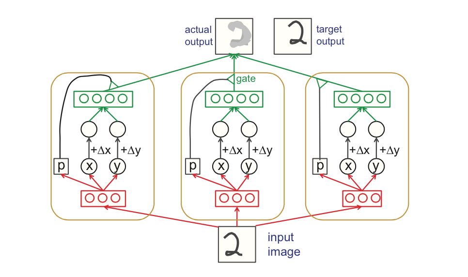
One of the earlier figures explaining capsules and routing between them. Source.
As I showed in Part II, a capsule $i$ in a lower-level layer needs to decide how to send its output vector to higher-level capsules $j$. It makes this decision by changing scalar weight $c_{ij}$ that will multiply its output vector and then be treated as input to a higher-level capsule. Notation-wise, $c_{ij}$ represents the weight that multiplies output vector from lower-level capsule $i$ and goes as input to a higher level capsule $j$.
Things to know about weights $c_{ij}$:
- Each weight is a non-negative scalar
- For each lower level capsule $i$, the sum of all weights $c_{ij}$ equals to 1
- For each lower level capsule $i$, the number of weights equals to the number of higher-level capsules
- These weights are determined by the iterative dynamic routing algorithm
The first two facts allow us to interpret weights in probabilistic terms. Recall that the length a capsule’s output vector is interpreted as probability of existence of the feature that this capsule has been trained to detect. Orientation of the output vector is the parametrized state of the feature. So, in a sense, for each lower level capsule $i$, its weights $c_{ij}$ define a probability distribution of its output belonging to each higher level capsule $j$.
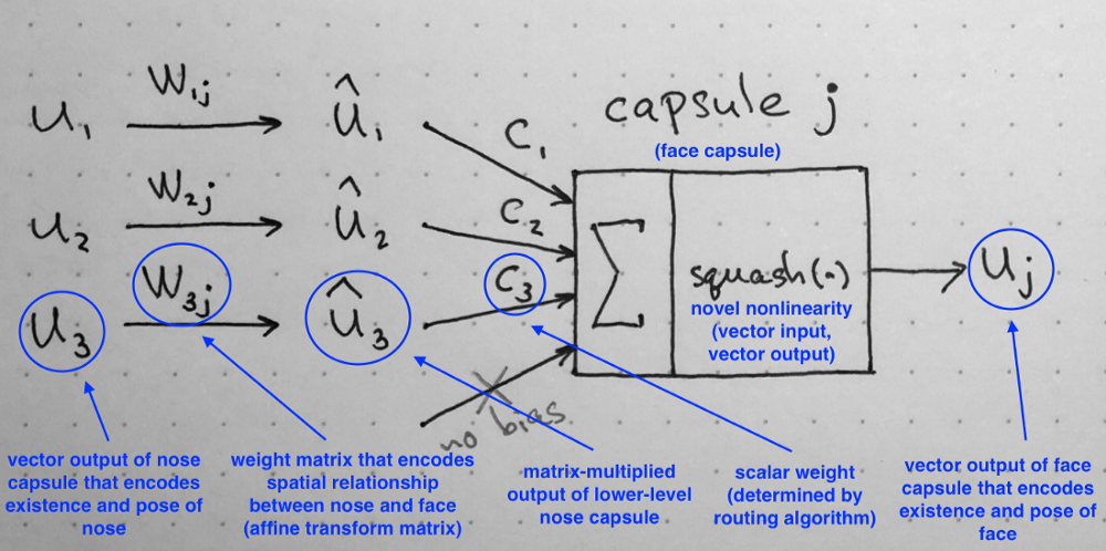
Recall: computations inside of a capsule as described in Part II of the series. Source: author.
Dynamic Routing Between Capsules
So, what exactly happens during dynamic routing? Let’s have a look at the description of the algorithm as published in the paper. But before we dive into the algorithm step by step, I want you to keep in your mind the main intuition behind the algorithm:
Lower level capsule will send its input to the higher level capsule that “agrees” with its input. This is the essence of the dynamic routing algorithm.
Now that we have this in mind, let’s go through the algorithm line by line.
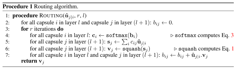
Dynamic routing algorithm, as published in the original paper.
The first line says that this procedure takes all capsules in a lower level $l$ and their outputs $\hat{u}$, as well as the number of routing iterations $r$. The very last line tells you that the algorithm will produce the output of a higher level capsule $v_j$. Essentially, this algorithm tells us how to calculate forward pass of the network.
In the second line you will notice that there is a new coefficient $b_{ij}$ that we haven’t seen before. This coefficient is simply a temporary value that will be iteratively updated and, after the procedure is over, its value will be stored in $c_{ij}$. At start of training the value of $b_{ij}$ is initialized at zero.
Line 3 says that the steps in 4–7 will be repeated $r$ times (the number of routing iterations).
Step in line 4 calculates the value of vector $c_i$ which is all routing weights for a lower level capsule $i$. This is done for all lower level capsules. Why softmax? Softmax will make sure that each weight $c_{ij}$ is a non-negative number and their sum equals to one. Essentially, softmax enforces probabilistic nature of coefficients $c_{ij}$ that I described above.
At the first iteration, the value of all coefficients $c_{ij}$ will be equal, because on line two all $b_{ij}$ are set to zero. For example, if we have 3 lower level capsules and 2 higher level capsules, then all $c_{ij}$ will be equal to 0.5. The state of all $c_{ij}$ being equal at initialization of the algorithm represents the state of maximum confusion and uncertainty: lower level capsules have no idea which higher level capsules will best fit their output. Of course, as the process is repeated these uniform distributions will change.
After all weights $c_{ij}$ were calculated for all lower level capsules, we can move on to line 5, where we look at higher level capsules. This step calculates a linear combination of input vectors, weighted by routing coefficients $c_{ij}$, determined in the previous step. Intuitively, this means scaling down input vectors and adding them together, which produces output vector $s_j$. This is done for all higher level capsules.
Next, in line 6 vectors from last step are passed through the squash nonlinearity, that makes sure the direction of the vector is preserved, but its length is enforced to be no more than 1. This step produces the output vector $v_j$ for all higher level capsules.
To summarize what we have so far: steps 4–6 simply calculate the output of higher level capsules. Step on line 7 is where the weight update happens. This step captures the essence of the routing algorithm. This steps looks at each higher level capsule $j$ and then examines each input and updates the corresponding weight $b_{ij}$ according to the formula. The formula says that the new weight value equals to the old value plus the dot product of current output of capsule $j$ and the input to this capsule from a lower level capsule $i$. The dot product looks at similarity between input to the capsule and output from the capsule. Also, remember from above, the lower level capsule will sent its output to the higher level capsule whose output is similar. This similarity is captured by the dot product. After this step, the algorithm starts over from step 3 and repeats the process $r$ times.
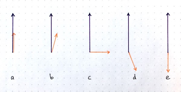
Dot product is an operation that takes 2 vectors and outputs a scalar. There are several scenarios possible for the two vectors of given lengths but different relative orientations: (a) largest positive possible values; (b) positive dot product; (c) zero dot product; (d) negative dot product; (e) largest possible negative dot product. You can think of the dot product as a measure of similarity in the context of CapsNets. Source: author.
After $r$ times, all outputs for higher level capsules were calculated and routing weights have been established. The forward pass can continue to the next level of network.
Intuitive Example of Weight Update Step
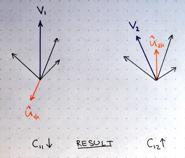
Two higher level capsules with their outputs represented by purple vectors, and inputs represented by black and orange vectors. Lower level capsule with orange output will decrease the weight for higher level capsule 1 (left side) and increase the weight for higher level capsule 2 (right side). Source: author.
In the figure above, imagine that there are two higher level capsules, their output is represented by purple vectors $v_1$ and $v_2$ calculated as described in previous section. The orange vector represents input from one of the lower level capsules and the black vectors represent all the remaining inputs from other lower level capsules.
We see that in the left part the purple output $v_1$ and the orange input $\hat{u}$ point in the opposite directions. In other words, they are not similar. This means their dot product will be a negative number and as result routing coefficient $c_{11}$ will decrease. In the right part, the purple output $v_2$ and the orange input $\hat{v}$ point in the same direction. They are similar. Therefore, the routing coefficient $c_{12}$ will increase. This procedure is repeated for all higher level capsules and for all inputs of each capsule. The result of this is a set of routing coefficients that best matches outputs from lower level capsules with outputs of higher level capsules.
How Many Routing Iterations to Use?
The paper examined a range of values for both MNIST and CIFAR data sets. Author’s conclusion is two-fold:
- More iterations tends to overfit the data
- It is recommended to use 3 routing iterations in practice
Conclusion
In this article, I explained the dynamic routing algorithm by agreement that allows to train the CapsNet. The most important idea is that similarity between input and output is measured as dot product between input and output of a capsule and then routing coefficient is updated correspondingly. Best practice is to use 3 routing iterations.
In the next post, I will walk you through CapsNet architecture, where we will put together all pieces of the puzzle that we learned so far.