Part of Understanding Hinton’s Capsule Networks Series:
- Part 1: Intuition
- Part 2: How Capsules Work
- Part 3: Dynamic Routing Between Capsules
- Part 4: CapsNet Architecture (you are reading it now)
Introduction
In this part, I will walk through the architecture of the CapsNet. I will also offer my shot at calculating the number of trainable parameters in the CapsNet. My resulting number is around 8.2 million of trainable parameters which is different from the 11.36 officially referred to in the paper. The paper itself is not very detailed and hence it leaves some open questions about specifics of the network implementation that are as of today still unanswered because the authors did not provide their code. Nonetheless, I still think that counting parameters in a network is a good exercise for purely learning purposes as it allows one to practice understanding of all building blocks of a particular architecture.
The CapsNet has 2 parts: encoder and decoder. The first 3 layers are encoder, and the second 3 are decoder:
- Layer 1. Convolutional layer
- Layer 2. PrimaryCaps layer
- Layer 3. DigitCaps layer
- Layer 4. Fully connected #1
- Layer 5. Fully connected #2
- Layer 6. Fully connected #3
Part I. Encoder.
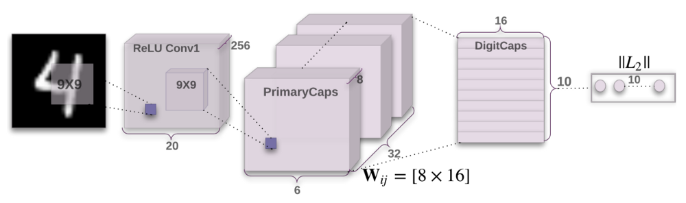
CapsNet encoder architecture. Source: original paper.
Encoder part of the network takes as input a 28 by 28 MNIST digit image and learns to encode it into a 16-dimensional vector of instantiation parameters (as explained in the previous posts of this series), this is where the capsules do their job. The output of the network during prediction is a 10-dimensional vectors of lengths of DigitCaps’ outputs. The decoder has 3 layers: two of them are convolutional and the last one is fully connected.
Layer 1. Convolutional layer
- Input: 28x28 image (one color channel).
- Output: 20x20x256 tensor.
- Number of parameters: 20992.
Convolutional layer’s job is to detect basic features in the 2D image. In the CapsNet, the convolutional layer has 256 kernels with size of 9x9x1 and stride 1, followed by ReLU activation. If you don’t know what this means, here are some awesome resources that will allow you to quickly pick up key ideas behind convolutions. To calculate the number of parameters, we need to also remember that each kernel in a convolutional layer has 1 bias term. Hence this layer has (9x9 + 1)x256 = 20992 trainable parameters in total.
Layer 2. PrimaryCaps layer
- Input: 20x20x256 tensor.
- Output: 6x6x8x32 tensor.
- Number of parameters: 5308672.
This layer has 32 primary capsules whose job is to take basic features detected by the convolutional layer and produce combinations of the features. The layer has 32 “primary capsules” that are very similar to convolutional layer in their nature. Each capsule applies eight 9x9x256 convolutional kernels (with stride 2) to the 20x20x256 input volume and therefore produces 6x6x8 output tensor. Since there are 32 such capsules, the output volume has shape of 6x6x8x32. Doing calculation similar to the one in the previous layer, we get 5308672 trainable parameters in this layer.
Layer 3. DigitCaps layer
- Input: 6x6x8x32 tensor.
- Output: 16x10 matrix.
- Number of parameters: 1497600.
This layer has 10 digit capsules, one for each digit. Each capsule takes as input a 6x6x8x32 tensor. You can think of it as 6x6x32 8-dimensional vectors, which is 1152 input vectors in total. As per the inner workings of the capsule (as described here), each of these input vectors gets their own 8x16 weight matrix that maps 8-dimensional input space to the 16-dimensional capsule output space. So, there are 1152 matrices for each capsule, and also 1152 c coefficients and 1152 b coefficients used in the dynamic routing. Multiplying: 1152 x 8 x 16 + 1152 + 1152, we get 149760 trainable parameters per capsule, then we multiply by 10 to get the final number of parameters for this layer.
The loss function
The loss function might look complicated at first sight, but it really is not. It is very similar to the SVM loss function. In order to understand the main idea about how it works, recall that the output of the DigitCaps layer is 10 sixteen-dimensional vectors. During training, for each training example, one loss value will be calculated for each of the 10 vectors according to the formula below and then the 10 values will be added together to calculate the final loss. Because we are talking about supervised learning, each training example will have the correct label, in this case it will be a ten-dimensional one-hot encoded vector with 9 zeros and 1 one at the correct position. In the loss function formula, the correct label determines the value of $T_c$: it is 1 if the correct label corresponds with the digit of this particular DigitCap and 0 otherwise.
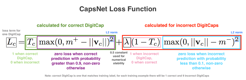
Color coded loss function equation. Source: author, based on original paper.
Suppose the correct label is 1, this means the first DigitCap is responsible for encoding the presence of the digit 1. For this DigitCap’s loss function $T_c$ will be one and for all remaining nine DigitCaps $T_c$ will be 0. When $T_c$ is 1 then the first term of the loss function is calculated and the second becomes zero. For our example, in order to calculate the first DigitCap’s loss we take the output vector of this DigitCap and subtract it from $m+$, which is fixed at 0.9. Then we keep the resulting value only in the case when it is greater than zero and square it. Otherwise, return 0. In other words, the loss will be zero if the correct DigitCap predicts the correct label with greater than 0.9 probability, and it will be non-zero if the probability is less than 0.9.
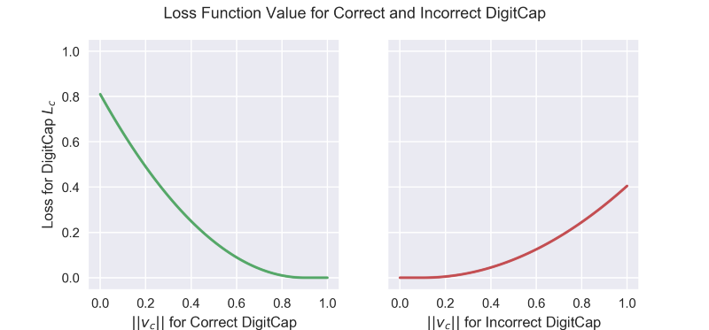
Loss function value for correct and incorrect DigitCap. Note that the red graph is “squashed” vertically compared to the green one. This is due to the lambda multiplier from the formula. Source: author.
For DigitCaps who do not match with the correct label, $T_c$ will be zero and therefore the second term will be evaluated (corresponding to $(1 — T_c)$ part). In this case we can see that the loss will be zero if the mismatching DigitCap predicts an incorrect label with probability less than 0.1 and non-zero if it predicts an incorrect label with probability more than 0.1.
Finally, in the formula lambda coefficient is included for numerical stability during training (its value is fixed at 0.5). The two terms in the formula have squares because this loss function has $L_2$ norm and the authors apparently consider this norm to work better.
Part II. Decoder.
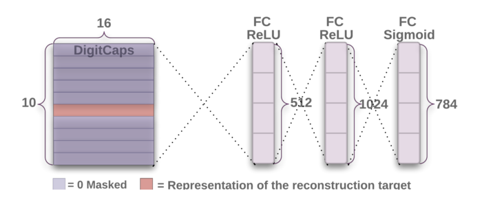
CapsNet decoder architecture. Source: original paper.
Decoder takes a 16-dimensional vector from the correct DigitCap and learns to decode it into an image of a digit (note that it only uses the correct DigitCap vector during training and ignores the incorrect ones). Decoder is used as a regularizer, it takes the output of the correct DigitCap as input and learns to recreate an 28 by 28 pixels image, with the loss function being Euclidean distance between the reconstructed image and the input image. Decoder forces capsules to learn features that are useful for reconstructing the original image. The closer the reconstructed image to the input image, the better. Examples of reconstructed images can be seen in the image below.
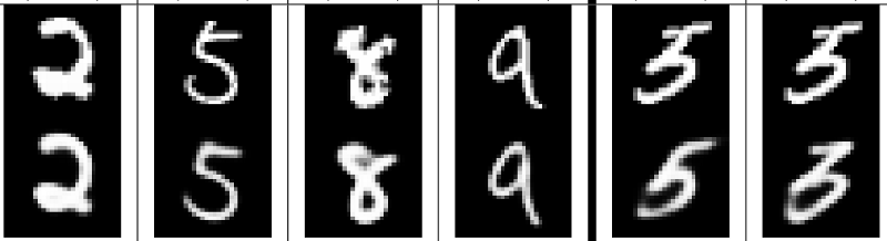
Top row: original images. Bottom row: reconstructed images. Source: original paper.
Layer 4. Fully connected #1
- Input: 16x10.
- Output: 512.
- Number of parameters: 82432.
Each output of the lower level gets weighted and directed into each neuron of the fully connected layer as input. Each neuron also has a bias term. For this layer there are 16x10 inputs that are all directed to each of the 512 neurons of this layer. Therefore, there are (16x10 + 1)x512 trainable parameters.
For the following two layers calculation is the same: number of parameters = (number of inputs + bias) x number of neurons in the layer. This is why there is no explanation for fully connected layers 2 and 3.
Layer 5. Fully connected #2
- Input: 512.
- Output: 1024.
- Number of parameters: 525312.
Layer 6. Fully connected #3
- Input: 1024.
- Output: 784 (which after reshaping gives back a 28x28 decoded image).
- Number of parameters: 803600.
Total number of parameters in the network: 8238608.
Conclusion
This wraps up the series on the CapsNet. There are many very good resources around the internet. If you would like to learn more on this fascinating topic, please have a look at this awesome compilation of links about CapsNets.