In this article, I will discuss two interesting recent papers that provide an easy way to improve performance of any given neural network by using a smart way to ensemble. They are:
- “Loss Surfaces, Mode Connectivity, and Fast Ensembling of DNNs” by Garipov et. al
- “Averaging Weights Leads to Wider Optima and Better Generalization” by Izmailov et. al
Additional prerequisite reading that will make context of this post much more easy to understand:
- “Improving the way we work with learning rate” by Vitaly Bushaev
Traditional Ensembling of Neural Networks
Traditional ensembling combines several different models and makes them predict on the same input. Then some way of averaging is used to determine the final prediction of the ensemble. It can be simple voting, an average or even another model that learns to predict correct value or label based on the inputs of models in the ensemble. Ridge regression is one particular way of combining several predictions which is used by Kaggle-winning machine learning practitioners.
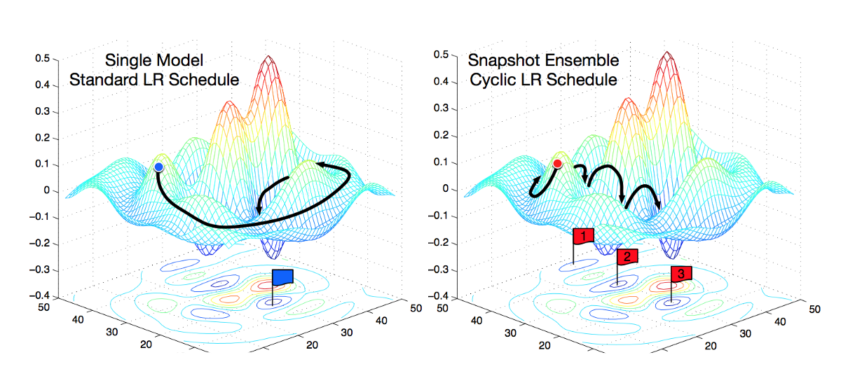
Snapshot Ensemble is created by saving a model each time the learning rate cycle is at the end. Then the saved models are used together during prediction. Source.
When applied in deep learning, ensembling can be used to combine predictions of several neural networks to produce one final prediction. Usually it is a good idea to use neural networks of different architectures in an ensemble, because they will likely make mistakes on different training samples and therefore the benefit of ensembling will be larger.
However, you can also ensemble models with the same architecture and it will give surprisingly good results. One very cool trick exploiting this approach was proposed in the snapshot ensembling paper. The authors take weights snapshot while training the same network and then after training create an ensemble of nets with the same architecture but different weights. This allows to improve test performance, and it is a very cheap way too because you just train one model once, just saving weights from time to time.
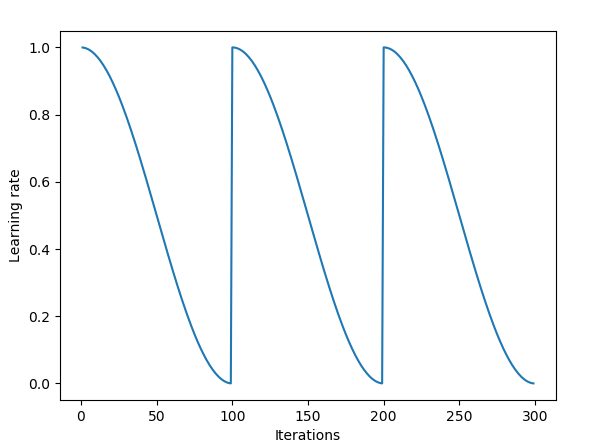
Snapshot ensemble uses cyclical learning rates with annealing. Source.
You can refer to this awesome post for more details. If you aren’t yet using cyclical learning rates, then you definitely should, as it becomes the standard state-of-the art training technique that is very simple, not computationally heavy and provides significant gains at almost no additional cost.
All of the examples above are ensembles in the model space, because they combine several models and then use models’ predictions to produce the final prediction.
In the paper that I am discussing in this post, however, the authors propose to use a novel ensembling in the weights space. This method produces an ensemble by combining weights of the same network at different stages of training and then uses this model with combined weights to make predictions. There are 2 benefits from this approach:
- when combining weights, we still get one model at the end, which speeds up predictions
- it turns out, this method beats the current state-of-the art snapshot ensembling
Let’s see how it works. But first we need to understand some important facts about loss surfaces and generalizable solutions.
Solutions in the Weight Space
The first important insight is that a trained network is a point in multidimensional weight space. For a given architecture, each distinct combination of network weights produces a separate model. Since there are infinitely many combinations of weights for any given architecture, there will be infinitely many solutions. The goal of training of a neural network is to find a particular solution (point in the weight space) that will provide low value of the loss function both on training and testing data sets.
During training, by changing weights, training algorithm changes the network and travel in the weight space. Gradient descent algorithm travels on a loss plane in this space where plane elevation is given by the value of the loss function.
Narrow and Wide Optima
It is very hard to visualize and understand the geometry of multidimensional weight space. At the same time, it is very important to understand it because stochastic gradient descent essentially traverses a loss surface in this highly multidimensional space during training and tries to find a good solution — a “point” on the loss surface where loss value is low. It is known that such surfaces have many local optima. But it turns out that not all of them are equally good.
Hinton: “To deal with hyper-planes in a 14-dimensional space, visualize a 3-D space and say “fourteen” to yourself very loudly. Everyone does it.” (source)
One metric that can distinguish a good solution from a bad one is its flatness. The idea being that training data set and testing data set will produce similar but not exactly the same loss surfaces. You can imagine that a test surface will be shifted a bit relative to the train surface. For a narrow solution, during test time, a point that gave low loss can have a large loss because of this shift. This means that this “narrow” solution did not generalize well — training loss is low, while testing loss is large. On the other hand, for a “wide” and flat solution, this shift will lead to training and testing loss being close to each other.
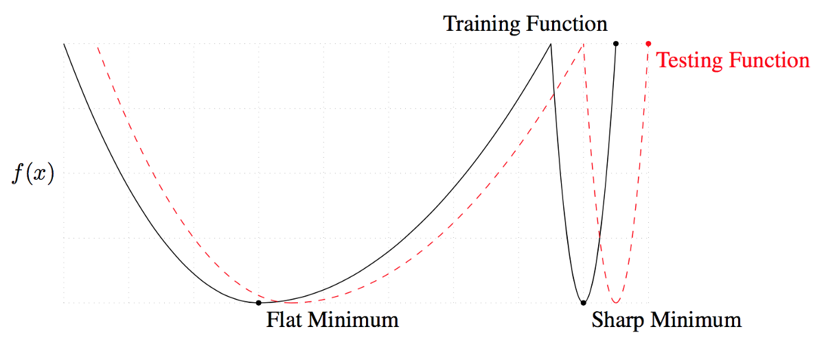
Narrow and wide optima. Flat minimum will produce similar loss during training and testing. Narrow loss, however, will give very different results during training and testing. In other words, wide minimum is more generalizable than narrow. Source.
I explained the difference between narrow and wide solutions because the new method which is the focus of this post leads to nice and wide solutions.
Snapshot Ensembling
Initially, SGD will make a big jump in the weight space. Then, as the learning rate gets smaller due to cosine annealing, SGD will converge to some local solution and the algorithm will take a “snapshot” of the model by adding it to the ensemble. Then the rate is reset to high value again and SGD takes a large jump again before converging to some different local solution.
Cycle length in the snapshot ensembling approach is 20 to 40 epochs. The idea of long learning rate cycles is to be able to find sufficiently different models in the weight space. If the models are too similar, then predictions of the separate networks in the ensemble will be too close and the benefit of ensembling will be negligible.
Snapshot ensembling works really well and improves model performance, but Fast Geometric Ensembling works even better.
Fast Geometric Ensembling (FGE)
Fast geometric ensembling is very similar to snapshot ensembling, but is has some distinguishing features. It uses linear piecewise cyclical learning rate schedule instead of cosine. Secondly, the cycle length in FGE is much shorter — only 2 to 4 epochs per cycle. At first intuition, the short cycle is wrong because the models at the end of each cycle will be close to each other and therefore ensembling them will not give any benefits. However, as the authors discovered, because there exist connected paths of low loss between sufficiently different models, it is possible to travel along those paths in small steps and the models encountered along will be different enough to allow ensembling them with good results. Thus, FGE shows improvement compared to snapshot ensembles and it takes smaller steps to find the model (which makes it faster to train).
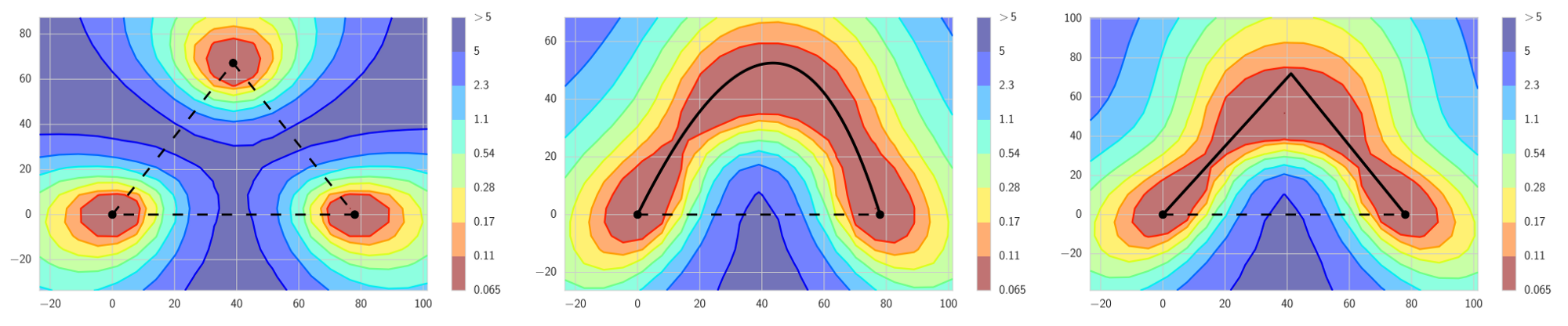
LEFT: Traditional intuition is that good local minima are separated by regions of high loss. This is true if we travel along the lines connecting local minima. MIDDLE and RIGHT: However, there exist paths between local minima, such that loss stays low on these paths. FGE takes snapshots along these paths and creates an ensemble out of the snapshots. Source.
To benefit from both snapshot ensembling or FGE, one needs to store multiple models and then make predictions for all of them before averaging for the final prediction. Thus, for additional performance of the ensemble, one needs to pay with higher amount of computation. So there is no free lunch there. Or is there? This is where the new paper with stochastic weight averaging comes in.
Stochastic Weight Averaging (SWA)
Stochastic weight averaging closely approximates fast geometric ensembling but at a fraction of computational loss. SWA can be applied to any architecture and data set and shows good result in all of them. The paper suggests that SWA leads to wider minima, the benefits of which I discussed above. SWA is not an ensemble in its classical understanding. At the end of training you get one model, but it’s performance beats snapshot ensembles and approaches FGE.
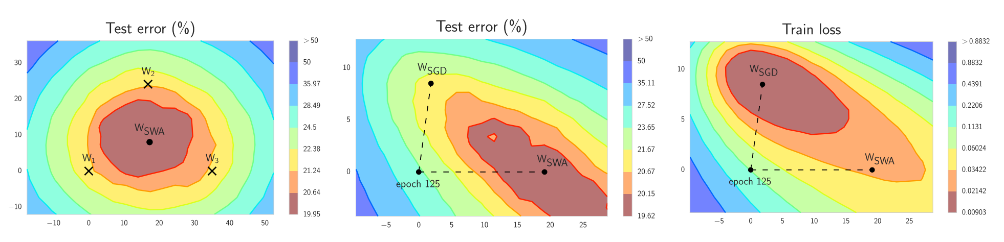
LEFT: $W_1$, $W_2$ and $W_3$ represent 3 independently trained networks, $W_{swa}$ is the average of them. MIDDLE: $W_{swa}$ provides superior performance on the test set as compared to SGD. RIGHT: Note that even though $W_{swa}$ shows worse loss during training, it generalizes better. Source.
Intuition for SWA comes from empirical observation that local minima at the end of each learning rate cycle tend to accumulate at the border of areas on loss surface where loss value is low (points $W_1$, $W_2$ and $W_3$ are at the border of the red area of low loss in the left panel of figure above). By taking the average of several such points, it is possible to achieve a wide, generalizable solution with even lower loss ($W_{SWA}$ in the left panel of the figure above).
Here is how it works. Instead of an ensemble of many models, you only need two models:
- the first model that stores the running average of model weights ($W_{SWA}$ in the formula). This will be the final model after the end of the training which will be used for predictions.
- the second model ($w$ in the formula) that will be traversing the weight space, exploring it by using a cyclical learning rate schedule.
At the end of each learning rate cycle, the current weights of the second model ($w$) will be used to update the weight of the running average model ($w_{SWA}$) by taking weighted mean between the old running average weights and the new set of weights from the second model:
\[w_{SWA} \leftarrow \frac{w_{SWA} \cdot n_{models} + w}{n_{models} + 1}\]By following this approach, you only need to train one model, and store only two models in memory during training. For prediction, you only need the running average model and predicting on it is much faster than using ensemble described above, where you use many models to predict and then average results.
Implementations
Authors of the paper provide their own implementation in PyTorch.
Also, SWA is implemented in the awesome fast.ai library that everyone should be using. And if you haven’t yet seen their course, then follow the links.