Architecture
AlexNet [2012, paper by Krizhevsky et al.]
Main Ideas
ReLU nonlinearity, training on multiple GPUs, local response normalization, overlapping pooling, data augmentation, dropout
Why it is Important
AlexNet won the ImageNet competition in 2012 by a large margin. It was the biggest network at the time. The network demonstrated the potential of training large neural networks quickly on massive datasets using widely available gaming GPUs; before that neural networks had been trained mainly on CPUs. AlexNet also used novel ReLU activation, data augmentation, dropout and local response normalization. All of these allowed to achieve state-of-the art performance in object recognition in 2012.
Brief Description
ReLU Nonlinearity
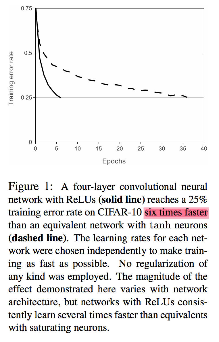
The benefits of ReLU (excerpt from the paper).
ReLU is a so-called non-saturating activation. This means that gradient will never be close to zero for a positive activation and as result, the training will be faster.
By contrast, sigmoid activations are saturating, which makes gradient close to zero for large absolute values of activations. Very small gradient will make the network train slower or even stop, because the step size during gradient descent’s weight update will be small or zero (so-called vanishing gradient problem).
By employing ReLU, training speed of the network was six times faster as compared to classical sigmoid activations that had been popular before ReLU. Today, ReLU is the default choice of activation function.
Local Response Normalization
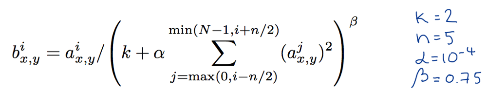
Local response normalization formula from the paper. Color labeling is mine.
After layers C1 and C2, activities of neurons were normalized according to the formula above. What this did is scaled the activities down by taking into account 5 neuron activities at preceding and following feature channels at the same spatial position.
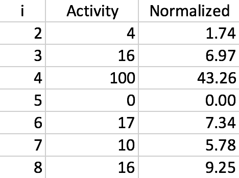
An example of local response normalization made in Excel by me.
These activities were squared and used together with parameters $n$, $k$, $\alpha$ and $\beta$ to scale down each neuron’s activity. Authors argue that this created “competition for big activities amongst neuron outputs computed using different kernels”. This approach reduced top-1 error by 1%. In the table above you can see an example of neuron activations scaled down by using this approach. Also note that the values of $n$, $k$, $\alpha$ and $\beta$ were selected using cross-validation.
Overlapping Pooling
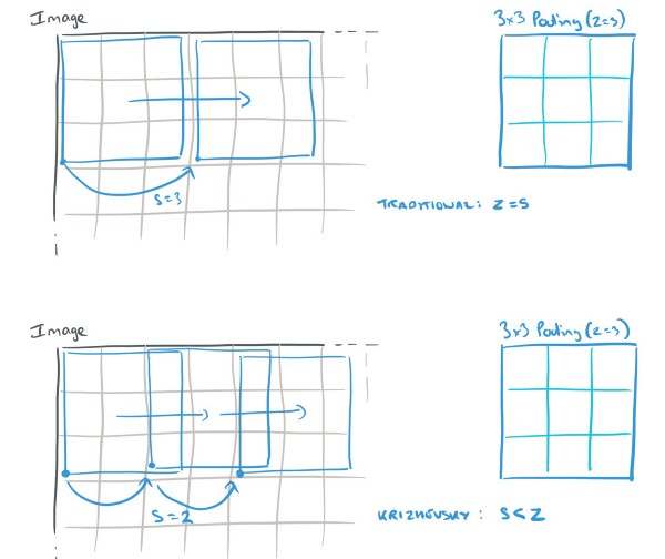
Overlapping pooling of the kind used by AlexNet. Source.
AlexNet used max pooling of size 3 and stride 2. This means that the largest values were pooled from 3x3 regions, centers of these regions being 2 pixels apart from each other vertically and horizontally. Overlapping pooling reduced tendency to overfit and also reduced test error rates by 0.4% and 0.3% (for top-1 and top-5 error correspondingly).
Data Augmentation
Data augmentation is a regularization strategy (a way to prevent overfitting). AlexNet uses two data augmentation approaches.
The first takes random crops of input images, as well as rotations and flips and uses them as inputs to the network during training. This allows to vastly increase the size of the data; the authors mention the increase by the factor of 2048. Another benefit is the fact that augmentation is performed on the fly on CPU while the GPUs train previous batch of data. In other words, this type of augmentation is essentially computationally free, and also does not require to store augmented images on disk.
The second data augmentation strategy is so-called PCA color augmentation. First, PCA on all pixels of ImageNet training data set is performed (a pixel is treated as a 3-dimensional vector for this purpose). As result, we get a 3x3 covariance matrix, as well as 3 eigenvectors and 3 eigenvalues. During training, a random intensity factor based on PCA components is added to each color channel of an image, which is equivalent to changing intensity and color of illumination. This scheme reduces top-1 error rate by over 1% which is a significant reduction.
Test Time Data Augmentation
The authors do not explicitly mention this as contribution of their paper, but they still employed this strategy. During test time, 5 crops of original test image (4 corners and center) are taken as well as their horizontal flips. Then predictions are made on these 10 images. Predictions are averaged to make the final prediction. This approach is called test time augmentation (TTA). Generally, it does not need to be only corners, center and flips, any suitable augmentation will work. This improves testing performance and is a very useful tool for deep learning practitioners.
Dropout
AlexNet used 0.5 dropout during training. This means that during forward pass, 50% of all activations of the network were set to zero and also did not participate in backpropagation. During testing, all neurons were active and were not dropped. Dropout reduces “complex co-adaptations” of neurons, preventing them to depend heavily on other neurons being present. Dropout is a very efficient regularization technique that makes the network learn more robust internal representations, significantly reducing overfitting.
Architecture
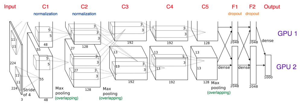
AlexNet architecture from paper. Color labeling is mine.
Architecture itself is relatively simple. There are 8 trainable layers: 5 convolutional and 3 fully connected. ReLU activations are used for all layers, except for the output layer, where softmax activation is used. Local response normalization is used only after layers C1 and C2 (before activation). Overlapping max pooling is used after layers C1, C2 and C5. Dropout was only used after layers F1 and F2.
Due to the fact that the network resided on 2 GPUs, it had to be split in 2 parts that communicated only partially. Note that layers C2, C4 and C5 only received as inputs outputs of preceding layers that resided on the same GPU. Communication between GPUs only happened at layer C3 as well as F1, F2 and the output layer.
The network was trained using stochastic gradient descent with momentum and learning rate decay. In addition, during training, learning rate was decreased manually by the factor of 10 whenever validation error rate stopped improving.
Additional Readings
- Paper: Rectified Linear Units Improve Restricted Boltzmann Machines
- Paper: Dropout: A Simple Way to Prevent Neural Networks from Overfitting
- Quora: Why are GPUs well-suited to deep learning?
- Why are GPUs necessary for training Deep Learning models?
- Data Augmentation: How to use Deep Learning when you have Limited Data.
- Color intensity data augmentation: Fancy PCA (Data Augmentation) with Scikit-Image
- PCA Color Augmentation
- Since PCA in the paper is done on the whole entirety of ImageNet data set (or maybe subsample, but that is not mentioned), the data most probably will not fit in memory. In that case, incremental PCA may be used that performs PCA in batches. This thread is also useful in explaining how to do partial PCA without loading the whole data in memory.
- Test time augmentation
Return to all architectures
Note: this post was originally published on Medium.