Finding Lane Lines on the Road

Portfolio Project Report

Note: Code for this project can be found on my GitHub.

The goals / steps of this project are the following:

• Make a pipeline that finds lane lines on the road
• Reflect on your work in a written report

Reflection

1. Pipeline Description

In this project, I developed a simple pipeline to find road lanes. The pipeline has the following steps:

1. Convert the original image to grayscale
2. Apply Gaussian blur to the grayscale image, get a blurred image
3. Apply Canny edge detector to the blurred image, get a black image with white adges
4. Apply ROI (region of interest) mask to the edges image to remove all edges outside ROI
5. Apply Hough transform to the masked edges image, get a list of line points as output
6. Transform the Hough lines into left and right lane lines:
   • Discard lines with slopes close to 0 (slopes in range from -0.3 to 0.3)
   • Separate remaining lines in two groups by the sign of the slope
   • Average out slopes and intercepts for each group
   • Return average slopes and intercepts for the left and right lane lines
7. Draw average lane lines on the original image, such that they are only show inside ROI
8. Save the image

Below are the images that show how the pipeline transforms the original image, according to the steps described above:

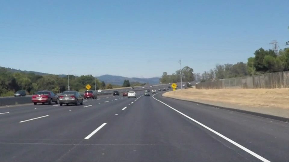
Step 1. Original image.

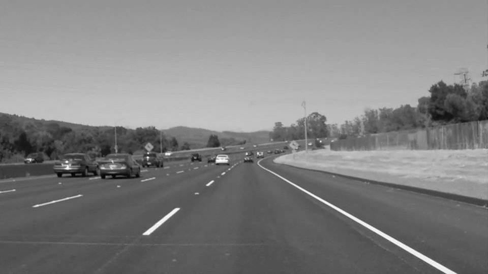
Step 2. Grayscale image.

Step 3. Blurred grayscale image.

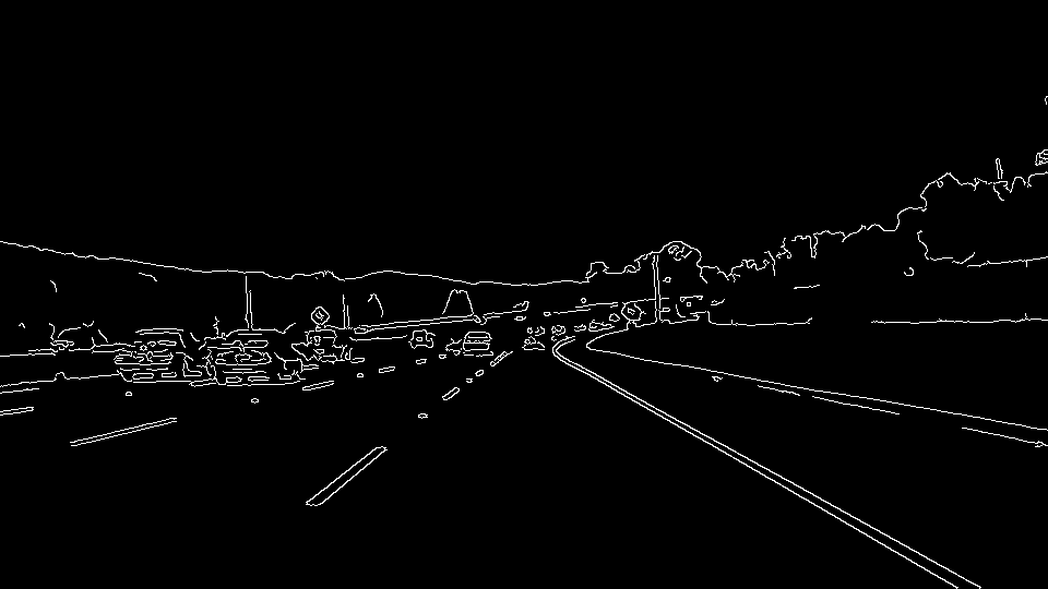
Step 4. Canny edges.

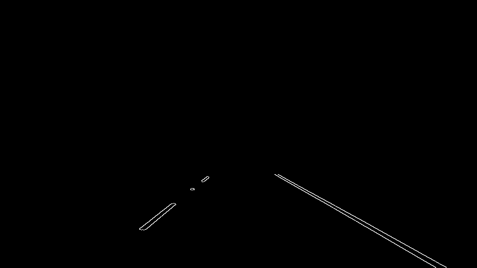
Step 5. ROI mask applied to Canny edges.

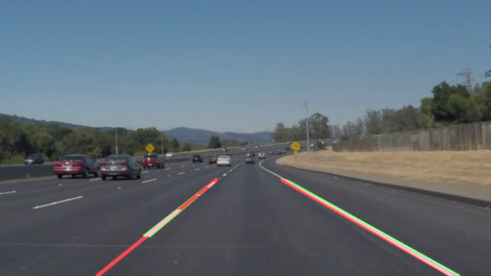
Step 6. Hough lines (green) and final averaged extrapolated lines (red).

In order to draw a single line on the left and right lanes, I modified the draw_lines() function by:

1. Separating Hough lines in two groups by slope (nagative and positive)
2. Removing lines with abnormal slopes (absolute value below 0.5 and above 1.5)
3. Averaging slopes and intercepts for each group
4. For average slope and intercepts, calculating the start and end points, such that lines are only drawn inside ROI
5. Adding lines to the original image

The most challenging parts were:

• finding optimal parameters for blur-Canny-Hough transformation
• deciding how to draw a single line for the left and the right lane lines

2. Potential Shortcomings of Current Pipeline

One potential shortcoming would be what would happen when the car is driving outside road lanes. In this case both lines will have the same slope and my pipeline will likely break down and will draw only one line.

Another shortcoming could be uneven color of the road surface, when there are tire markings on the road. By looking at the photo below, it can be seen that the current pipeling got confused, when the car drove on the patch of bright concrete with black tire marks. You can see multiple green Hough lines with very little slopes. They “pull” the average slopes and intercepts, so that the left and right red lines get really far from their normal positions.

The third shortcoming is that in the video, sometimes lines disappear for a fraction of a second. This means that the pipeline is unable to identify land lines for those frames. I think it is because of the parameters of the blur-Canny-Hough transform.

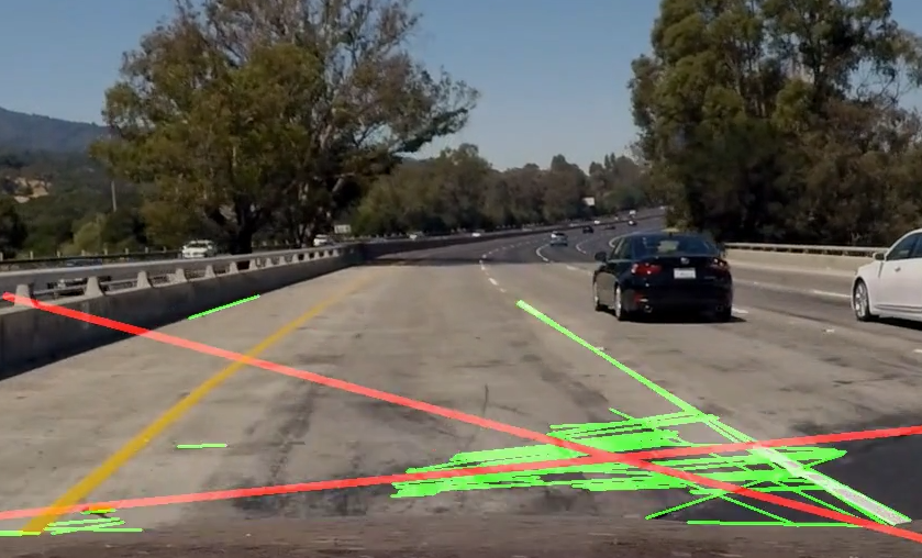
Confusing tire marks.

3. Possible Improvements of Pipeline

A possible improvement would be to develop a system to choose the best set of parameters for the pipeline in an automatic fashion.

Another improvement would be to dynamically change ROI depending on:

• road curvature
• whether the road slopes upward or downward
• speed of the vehicle

Yet another potential improvement could be to fit curves instead of the straight lines. This is especially important for turns, where lane lines are not straight, but curved.

In addition, I suggest “temporal smoothing” of lines to avoid erratic jumps from frame to frame. Basically, exponencial smoothing could help. In each new frame, the position of the line can be affected by the position in the previous frame and pipelines’ predictions for the current frame. By varying smoothing coefficient, it will make the jumps smaller.

I would also try to set up a deep learning system based on convolutional neural networks, collect some annotated data and train the network. I guess that reults would be much better, as CNN show to generalize well in computer vision tasks.

4. Conclusion

This project is really interesting, as the computer vision tools are useful knowledge and I feel like it would be beneficial do dig deeper. However, I see several shortcomings in the approach taken:

• multidimensional hyperparameter space for blur-Canny-Hough transform that is hard to search manually. Given the fact that parameters can drastically affect performance of the pipeline, there should be a better way to find the parameters
• the optimal set of parameters can depend on road conditions
• too many “hard-coded” decisions that would probably not generalize well

To summarize, I feel like a deep-learning-based approach would be more fruitful and generalizable.