Behavioral Cloning using Deep Learning

Portfolio Project Report

Note: Code for this project can be found on my GitHub.

1. Submission Files

My project includes the following files:

• model.py – the script used to create and train the final model.
• model.ipynb - the notebook used for development
• drive.py – the script provided by Udacity that is used to drive the car. I did not modify this script in any way.
• model.h5 – the saved model file. It can be used with Keras to load and compile the model.
• report.pdf – written report, that you are reading right now. It describes all the important steps done to complete the project.
• video.mp4 – video of the car, driving autonomously on the basic track.

2. Quality of Code

Originally, all of development for this project I did in Jupyter Notebook, because it is very easy to use in a trial-and-error setting. Before submitting the project, I took all the code from the notebook and put it into a file and named it model.py.

I split all the functionality used in this project into separate functions and defined them, providing a brief description of what each function does.

Even though the size of raw data is small enought to be stored in RAM on most modern computers, data augmentation techniques can quickly bloat really fast and make a computer slow. This happened to me in the early stages of this project. I quickly realized that this is not a good way to approach this problem and decided to use a generator to sequentially feed data in batches to the model. I made a generator that preprocesses and augments data in real time during training. This approach allows to use for training even large data sets that cannot comfortably fit into memory.

3. Model Architecture and Training Strategy

Before starting coding the model, I decided to do some research and read about architectures used by other people. I quckly noticed, that nVidia’s model was really popular. It was also relatively simple and not very expensive to train. So I started with that model. The model has:

1. Two preprocessing layers, which I will describe later when talking about data.
2. Three convolutional layers with (5,5) kernels (24, 26 and 48 kernels per layer, correspondingly) with (2,2) strides, followed by
3. Two convolutional layers with (3,3) kernels (64 kernels per layer) with (1,1) strides, followed by
4. Three fully connected layers (with 100, 50 and 10 neurons, correspondingly), followed by
5. Output layer with one output neuron that controls the steering wheel.

I decided to use ELU (Exponential Linear Unit) activation, because there is evidence that it can be slightly better than RELU. I did not notice any significant difference for my model, but it was already training really fast (around 70 seconds for roughly 14000 of images). All of the convolutional layers and all of the dense layers in my model with the exception of the last layer used ELU nonlinearity.

In order to train a model, I used two generators – one for training and one for validation. Validation data generator was used to assess out-of-sample performance. Training generator was performing random data augmentation to improve generalization capabilities of the model, but validation generator was only performing preprocessing without doing any of the augmentation. I will discuss augmentation procedures further below.

Because essentially the model was performing regression, the most appropriate evaluation metric was mean squre error ('mse' in Keras). The only problem with that metric is that it is unclear what it means in the context of driving a car autonomously. This metric, in other words, is not very intuitive. The only rule is the smaller, the better. The optimizer used in the model was an adaptive optimizer Adam with the default parameters.

When training the model as described in nVidia paper, I noticed that training error quickly was becoming smaller than validation error, which is the sign of overfitting. To reduce that I introduced dropout layers after each convolutional and each dense layer with the exception of the output layer. After training the model with different values of dropout I stopped at 0.5 for the final model.

The final architecture is presented in the table below.

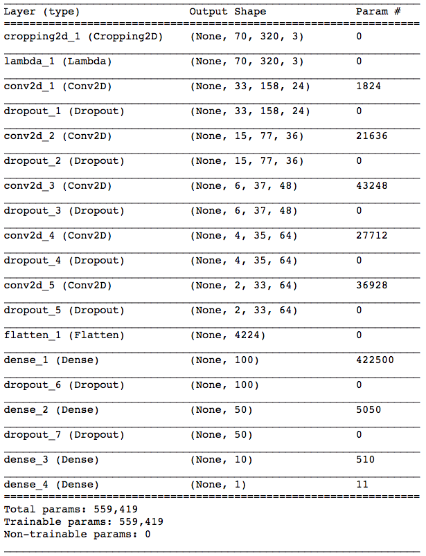
Architecture of deep network used for behavioral cloning.

I must admit that architecture-wise, this project is rather easy, especially with Keras that does all the shape inference for you automatically. The secret sauce in making the car drive itself well is not so much the architecture, but the data.

4. Data

A machine learning model is only as good as the data you put in. This is why data collection and processing is one of the most important parts of a successful machine learning application. In the following part I will address the issues related to data collection, preprocessing and augmentation. They were the key part of achieving good results in simulation.

4.1 Data Collection

As per Udacity suggestions, I collected two laps of “good smooth driving” in the center of the lane and one lap of “recoveries”, where I was placing the car in an undesired position away from the center of the road and then recorded the part when the car steers back to the center.

An iportant point is using keyboard vs. using controller. Analog controller allows to kee steering angle steady at some arbitrary fixed angle and that improves the quality of the data. I used controller to record laps of smooth driving but it was too cumbersome to record recoveries using controller, so I used keyboard instead.

4.2 Data Preprocessing

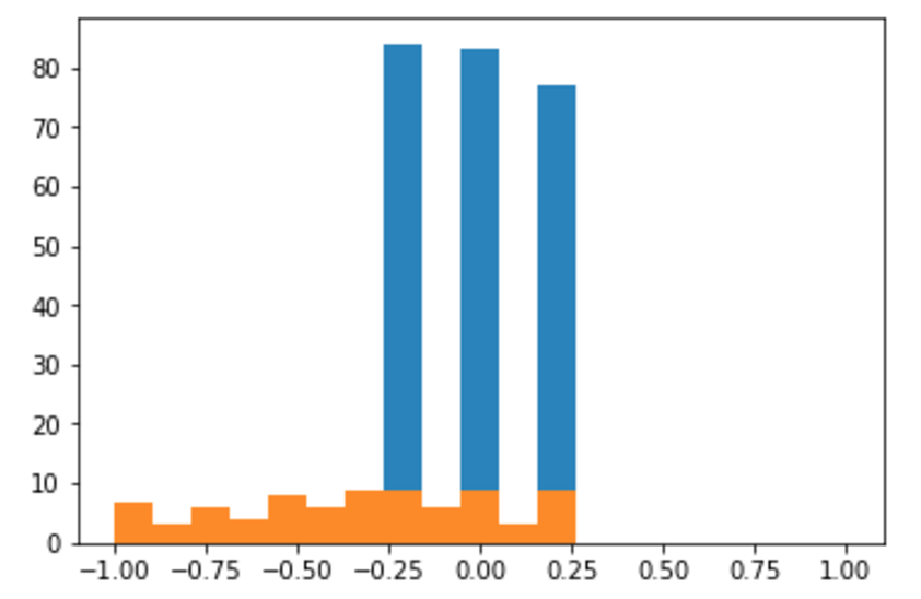
Horizontal axis: steering angle; vertical axis: number of training examples. Blue bars represent overrepresented classes, removed during data preprocessing step.

Challenges with the Project

Originally I thought that steps_per_epoch and validation_steps parameters of .fit_generator() method require the number of training examples. When I provided numbers of training examples, the training went extremely slow even though I was using a high-end GPU for training. At first, I thought I was hitting the hard drive read bottleneck, because my hard drive is old and slow. I tried to solve this problem by pre-loading all cleaned data into memory and then using that loaded data to pass to train generator and perform augmentation on the fly. I think that sped things up but just a little bit. After some time of frustration I finally realized that I was using steps_per_epoch and validation_steps parameters all wrong. I then adjusted the values of these parameters and the training started to be as fast as I expected given the speed of my GPU. I learned my lesson and will never forget what these two parameters mean.

I used generators of Keras before, for example flow_from_directory(), but I have never written my own custom generator. For some reason, I thought that it is too difficult and my level of Python was not advanced enough to write my own generators. I was mistaken and realized that generators are not that difficult. This was a really good practice and not only for Keras. Generators are widely used in Python and now I feel more confident in my ability to use and create them.