Portfolio Project Report
Note: Code for this project can be found on my GitHub.
The goals / steps of this project are the following:
- Compute the camera calibration matrix and distortion coefficients given a set of chessboard images.
- Apply a distortion correction to raw images.
- Use color transforms, gradients, etc., to create a thresholded binary image.
- Apply a perspective transform to rectify binary image (“birds-eye view”).
- Detect lane pixels and fit to find the lane boundary.
- Determine the curvature of the lane and vehicle position with respect to center.
- Warp the detected lane boundaries back onto the original image.
- Output visual display of the lane boundaries and numerical estimation of lane curvature and vehicle position.
Note: Most of the functionality for this project is contained in the file utils.py, provided with the project repo.
1. Camera Calibration
1. Briefly state how you computed the camera matrix and distortion coefficients. Provide an example of a distortion corrected calibration image.
The code used to compute camera calibration can be found in camera_calibration() method in utils.py.
This function loads all the test images of checkerboard provided by Udacity and uses cv2.findChessboardCorners() function to calculate calibration matrix and distances that I used later to undistort images. Out of 20 images of the checkerboard the alrorithm failed to identify points in 3 images. Those images contained the checkerboard that was partially outside the image region. All test images can be seen below. Note the 17 images with points drawn and 3 images without points:
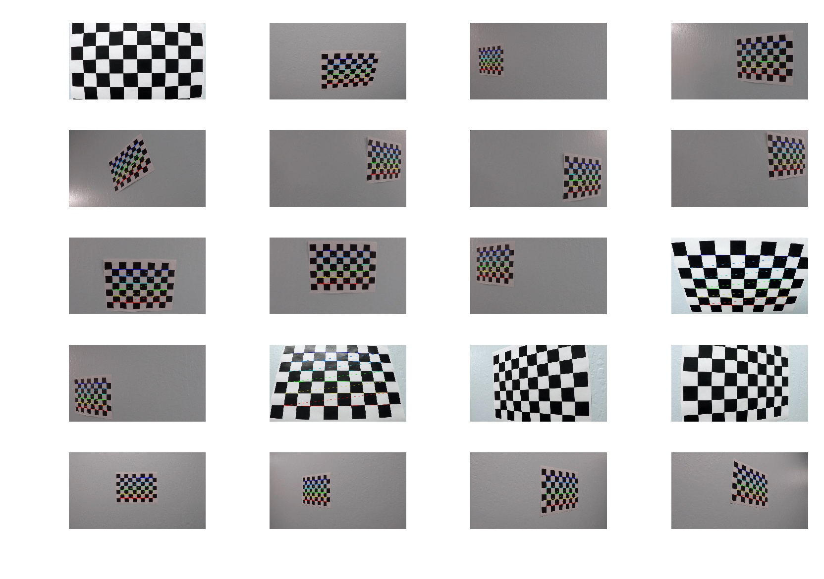
Camera calibration was performed on test images provided by Udacity. OpenCV was used for calibration.
After calibrating I tested whether it works on one of the images. I wrote undistort_image() function for this purpose.
It takes calibration matrix and distances vector produced in the previous step. Result can be seen below:
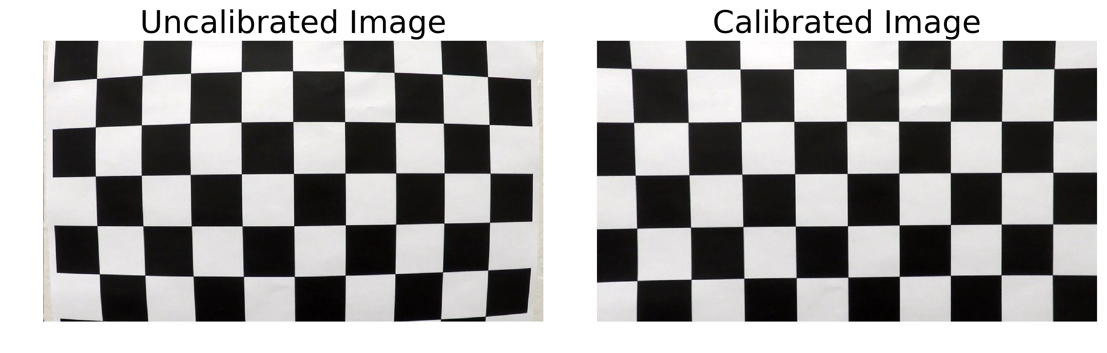
Clibration matrix applied to a distorted image (left) produces undistorted image (right).
It is clear that in the original image, some straight lines bend and are not in fact straight. In the processed image, however, lines are almost perfectly straight. Right angles are also right in the right image and hot so right in the left one. I think calibration could be improved had more images been used. Image undistortion is the first step in the pipeline.
2. Pipeline (single images)
The pipeline itself is coded in the notebook, but functionality wise everything is in the utils.py in class Pipeline.
The image / video processing pipeline had the following steps:
- Undistorting original image.
- Applying Gaussian blur.
- Creating thresholded binary image using color transform and Sobel filtering.
- Perspective transform to change into top-down view.
- Creating a sliding window mask in order filter out pixels unrelated to road lines.
- Applying the mask to the binary image.
- Fitting quadratic lines to the masked pixels.
- Prepare a top-down view colored overlay mask with road lines in blue and lane area in green.
- Putting colored mask onto original image (after unwarping it into camera view).
- Calculating distance from center line and road curvature and drawing them on image.
All these steps can be summarized graphically in the figure below:
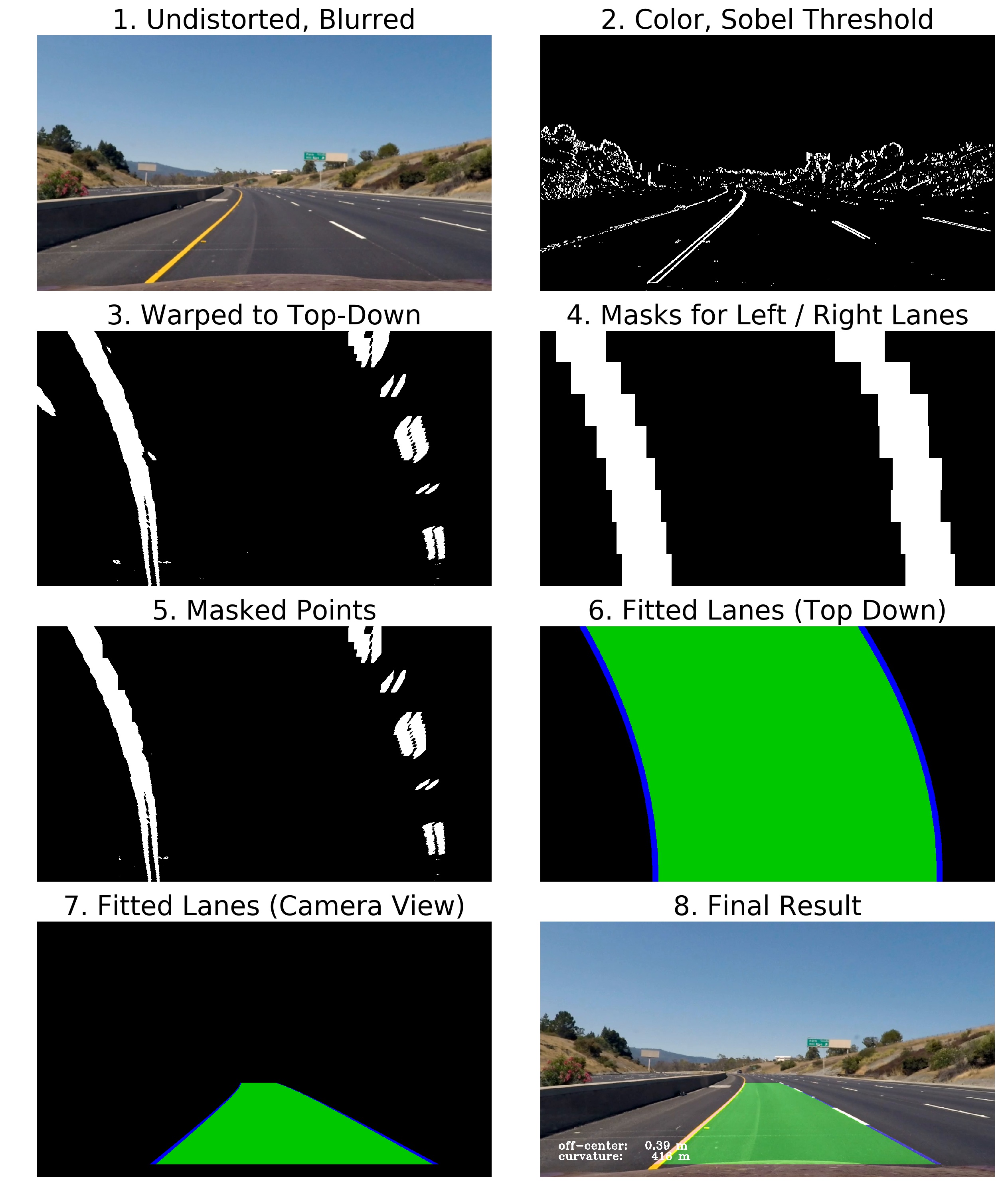
Full processing pipeline applied to a single frame.
Below I will briefly discuss all of the steps outline above.
1. Undistorting original image.
Every image was undistorted using camera calibration matrix and distances vector as described above.
2. Applying Gaussian blur.
Gaussian blur allows to reduce noise in the consequent stages and makes line fitting more robust. I used kernel size of 3. Method gaussian_blur() is used to apply this processing step.
Result of the first two steps can be seen in pipeline figure above in subplot 1.
3. Creating thresholded binary image using color transform and Sobel filtering.
This was the most challenging part of the whole pipeline. In order to get satisfactory results, I went through a lot of trial and error as well as incredible amount of frustration. I was even close to giving up on the project, but finally I was able to get a working combination of parameters. First, I tried the method offered in Udacity classroom but for some reason I was getiing very noisy masks that were very sensitive to shadows and light-grey sections of road. Then, I tried to use different combinations of Sobel thresholds, gradient direction and magnitude. It was not very successful. The problem here is there are a lot of parameters that can be tuned: min and max thresholds, different color spaces, x and y direction and so on. Hyperparameter space is very large and it is very hard to hit a good solution just by the method of trial and error. I researched and read numerous reports by other Udacity students and noticed that they all use different approaches that seem very random. There is no systematic approach to find a good solution.
At the end, I stopped at a simple combination of techniques. I noticed (Udacity also taught it), that S channel in HLS space can robustly identify yellow and white lanes. Light-grey sections of road cannot fool the S channel. The only problem is that it is not very robust with strong shadows, where it can have a lot of intensity in some areas.
To make it easier for the S channel threshold, I converted original image to gray and applied horizontal Sobel filter with kernel of 5. Then I performed thresholding. I used 175 for smallest value and 255 for largest. I also thresholded S channel with 30 for smallest and 150 for largest value. As result I had 2 binary masks. I combined them using or logical function to obtain the final binary image.
Functionality for this processing step can be found in combine_binary() method. This method calls some other smaller methods that can also be found in utils.py. Note that the method has more parameters that is uses. This is the remnant of the time when I tried different combinations of preprocessing steps.
Result can be seen in the pipeline figure in subplot 2.
4. Perspective transform to change into top-down view.
After getting binary image in the previous step, I applied perspective transform to it to change it from camera view into top-down view. To do that, I needed 2 sets of points: 4 points with coordinates in the original image and 4 points with the coordinates in the warped image. To get the source points, I wrote get_roi_vertices() method. It defines the coordinates based on percentages of height and width of the image. This approach allows to use images of any size, and relative positions of points will not change. Destination points in warped image are defined corners of the image in the method corners_unwarp() that also performs transformation itself.
This means that source points will fill the whole area of destination image. Destination image will have the same dimensions as the source image. Source and destination images can be seen in subplots 2 and 3, respectively, in the pipeline figure. The method uses cv2.getPerspectiveTransform() to get transform matrix and cv2.warpPerspective() to perform transform itself. It returns transformed image as well as the matrix for unwarping the image back into camera view later in the pipeline.
5. Creating a sliding window mask in order filter out pixels unrelated to road lines.
This part of the pipeline was also very challenging to implement in a robust way. The goal here is to create a mask for left and right road lines to only keep pixels of the lines and not anything esle. Implementation is in the method get_lanes_mask().
First, we get initial positions of lanes by using half of the image to calculate histogram and detect 2 peaks. Then, we split input image into horizontal strips (8 in this case). After that, for each strip, we try to detect two peaks, this is where centers of lanes are. Then we also create two empy (zero-valued) masks for left and right lane. For each peak we will take a 70 pixel window to each side of each peak and make this window one-valued in the mask. After we did this, we will have two masks that we can apply to the binary image from step 3.
After we have 2 fitted lines, we can simplify the search for masks. We can argue that lines in two consecutive frames will be close to each other. Therefore, the mask can be calculated as windows sitting on the fitted polynomial, which really speed up calculations.
In addition, if the algorithm fails to find peaks, window size can dynamically increase and then fall back to defauls when peaks were identified.
6. Applying the mask to the binary image.
After getting 2 masks for left and right lanes, we filter the binary image from step 3. In the fidure, you can see original binary image in subplot 3. Detected masks for both lines can be seen in subplot 4 and masked lines pixels can be seen in subplot 5. All functionality for this and previous steps can be found in the method get_lanes_mask(). The method returns masked images as well as the masks themselves. I needed masks so that I could produce pipeline visualization.
7. Fitting quadratic lines to the masked pixels.
This step was relatively easy. The code is in method fit_line(). It takes a masked binary images and calculates coordinates for all non-zero points. Then these point are used to fit a second-order polynomial using np.polyfit(). The tricky part was to rememeber that horizontal position is dependent variable and vertical is independent. In other words, we are fitting a function x = f(y) = a * y**2 + b * y + c (and not y = f(x) as we usually do in math).
Another trick that I used in this method is exponential smoothing. After receiving a new fir for the points in current frame, I also use fit from the last frame and calculate weighted sum of both, to produce the final fit. This has two benefits. First, this will remove the jiggle in the lines which is more aesthetically pleasing. Secondly, it makes the algorithm more robust, because if in some frame we will have some noise or maybe the mask algorithm finds bad masks, the resulting fit will still be close to the old one and the line will not jump to some weird place.
In addition, if no fit was found, the method falls back to the fit from the previous frame. The method returns a tuple of 3 coefficients for the second degree polynomial in the order of decreasing degree. I visualised fitted lines in subplot 6 in the pipeline figure. They are blue lines. Green area is just color filling between fitted lines to make it visually pleasing in the final video.
8. Prepare a top-down view colored overlay mask with road lines in blue and lane area in green.
After we get the points from the previous step, we can prepare colored mask to be overlaid on top of the original image. To do that, I created on emty 3-channel zero array and then used points and cv2 functions cv2.fillPoly() and cv2.polylines() to add green area and blue lines themselves. Result can be seen in subplot 6 of the figure. Functionality is in method prepare_lane_overlay() on line 694. The tricky part here was the order of points for drawing the green area. To do that, I had to flip points for one of the lines and them stack the points together. Method for doing that is prepare_poly_points().
9. Putting colored mask onto original image (after unwarping it into camera view).
This step is very straightforward. I used color overlay and the inverse transform matrix from step 4 to unwarp the overlay from top-down into camera view. Result can be seen in subplot 7. Then I used cv2.addWeighted() to combine the original image and the overlay, which can be seen in the last subplot.
10. Calculating distance from center line and road curvature and drawing them on image.
In addition to visually displaying the lines I aslo calculated off-center distance and road radius, as per Udacity project requirements. Both calculations are straightforward exercise in high school geometry and calculus. To calculate off-center distance I calculated distance on pixels from the center of the image to the center of the lane. Then I normalized distance in pixels into distance in meters by assuming that lane width is 3.7 meters.
The curvature was calculated according to the formula provided in the link by Udacity. It involved calculating the first and second derivatives for second-degree polynomial and plugging them in formula. The resulting value was in pixels, which I converted from pixels to meters.
Then I put the values on top of the image using cv2.putText() function. I also filtered out values too big for the radius, instead replacing them with straight string in the video. Methods for calculating off-center distance and radius of curvature are distance_from_center() and get_curvature().
Discussion
1. Briefly discuss any problems / issues you faced in your implementation of this project. Where will your pipeline likely fail? What could you do to make it more robust?
This project was much more challenging than I originally thought. The most chellenging part was figuring out an optimal binary image calculation approach. The challenge is to find such a combination of techniques that road lanes will be robustly detected no matter what lighting condition are present on road (light or shadow) and no matter what road surface is present on road (dark ashpalt or brighter concrete). I made a pipeline that works on this video. But of course it is not robust enough to work in more challenging conditions: night, shadows, snow, rain etc.
How can I make it more robust? I see two main ways to do that. First, is a better binary mask calculation. Second, is a better mask calculation approach. But I do not think these manual crafting approaches are the best.
I think that instead of trying to figure out the best set of hyperparameters by hand, it is better to let the computer figure it out automatically. Yes, I am talking about machine learning. I know there are neural nets that can detect and classify regions in an image. A network can be trained to distinguish road lanes very robustly. I think that advances in deep learning make this approach the best for this task. I would personally focus much more on deep learning for road lane detection if I was developing a self-driving car.
On the other hand, I learned a lot in this project about computer vision and image processing, so from this point of view this project is extermely useful for learning purposes.
Additional figure demonstrating the pipeline:
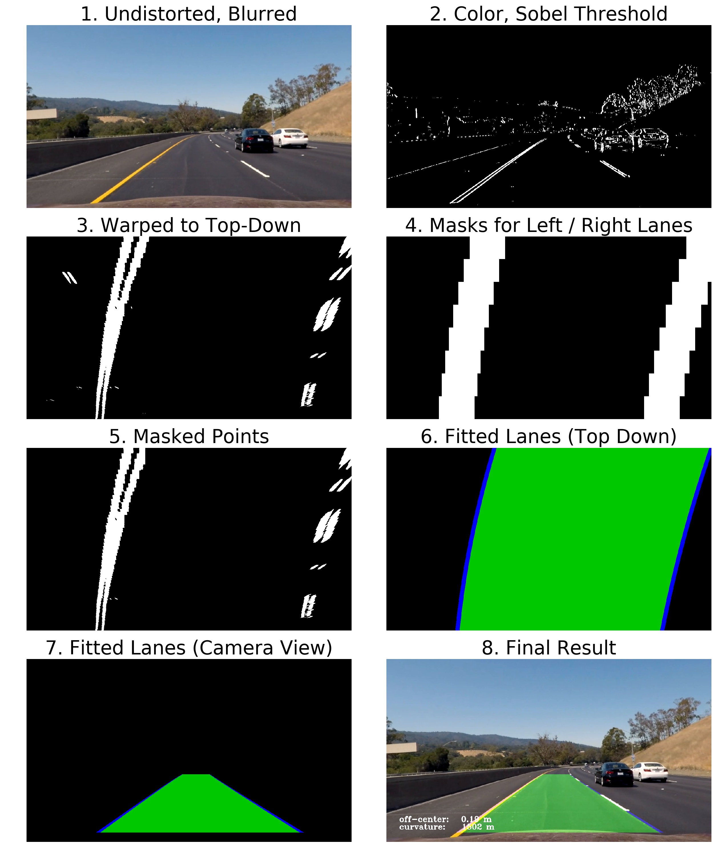
Full processing pipeline applied to another frame.