Part of Understanding Hinton’s Capsule Networks Series:
- Part 1: Intuition
- Part 2: How Capsules Work (you are reading it now)
- Part 3: Dynamic Routing Between Capsules
- Part 4: CapsNet Architecture
Introduction
In Part 1 of this series on capsule networks, I talked about the basic intuition and motivation behind the novel architecture. In this part, I will describe, what capsule is and how it works internally as well as intuition behind it. In the next part I will focus mostly on the dynamic routing algorithm.
What is a Capsule?
In order to answer this question, I think it is a good idea to refer to the first paper where capsules were introduced — “Transforming Autoencoders” by Hinton et al. The part that is important to understanding of capsules is provided below:
“Instead of aiming for viewpoint invariance in the activities of “neurons” that use a single scalar output to summarize the activities of a local pool of replicated feature detectors, artificial neural networks should use local “capsules” that perform some quite complicated internal computations on their inputs and then encapsulate the results of these computations into a small vector of highly informative outputs. Each capsule learns to recognize an implicitly defined visual entity over a limited domain of viewing conditions and deformations and it outputs both the probability that the entity is present within its limited domain and a set of “instantiation parameters” that may include the precise pose, lighting and deformation of the visual entity relative to an implicitly defined canonical version of that entity. When the capsule is working properly, the probability of the visual entity being present is locally invariant — it does not change as the entity moves over the manifold of possible appearances within the limited domain covered by the capsule. The instantiation parameters, however, are “equivariant” — as the viewing conditions change and the entity moves over the appearance manifold, the instantiation parameters change by a corresponding amount because they are representing the intrinsic coordinates of the entity on the appearance manifold.”
The paragraph above is very dense, and it took me a while to figure out what it means, sentence by sentence. Below is my version of the above paragraph, as I understand it:
Artificial neurons output a single scalar. In addition, CNNs use convolutional layers that, for each kernel, replicate that same kernel’s weights across the entire input volume and then output a 2D matrix, where each number is the output of that kernel’s convolution with a portion of the input volume. So we can look at that 2D matrix as output of replicated feature detector. Then all kernel’s 2D matrices are stacked on top of each other to produce output of a convolutional layer.
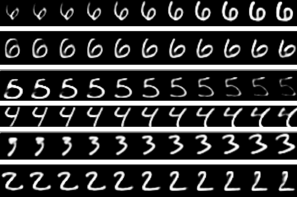
Not only can the CapsNet recognize digits, it can also generate them from internal representations. Source.
Then, we try to achieve viewpoint invariance in the activities of neurons. We do this by the means of max pooling that consecutively looks at regions in the above described 2D matrix and selects the largest number in each region. As result, we get what we wanted — invariance of activities. Invariance means that by changing the input a little, the output still stays the same. And activity is just the output signal of a neuron. In other words, when in the input image we shift the object that we want to detect by a little bit, networks activities (outputs of neurons) will not change because of max pooling and the network will still detect the object.
The above described mechanism is not very good, because max pooling loses valuable information and also does not encode relative spatial relationships between features. We should use capsules instead, because they will encapsulate all important information about the state of the features they are detecting in a form of a vector (as opposed to a scalar that a neuron outputs).
Capsules encapsulate all important information about the state of the feature they are detecting in vector form.
Capsules encode probability of detection of a feature as the length of their output vector. And the state of the detected feature is encoded as the direction in which that vector points to (“instantiation parameters”). So when detected feature moves around the image or its state somehow changes, the probability still stays the same (length of vector does not change), but its orientation changes.
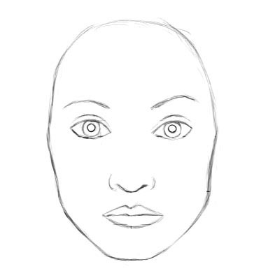
Imagine that a capsule detects a face in the image and outputs a 3D vector of length $0.99$. Then we start moving the face across the image. The vector will rotate in its space, representing the changing state of the detected face, but its length will remain fixed, because the capsule is still sure it has detected a face. This is what Hinton refers to as activities equivariance: neuronal activities will change when an object “moves over the manifold of possible appearances” in the picture. At the same time, the probabilities of detection remain constant, which is the form of invariance that we should aim at, and not the type offered by CNNs with max pooling.
How does a capsule work?
Let us compare capsules with artificial neurons. Table below summarizes the differences between the capsule and the neuron:
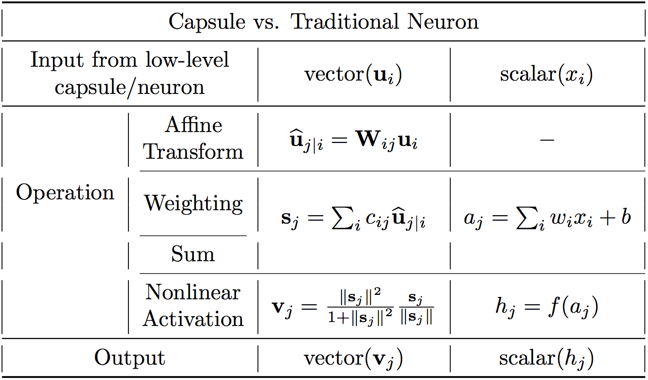
Important differences between capsules and neurons. Source: author, inspired by the talk on CapsNets given by naturomics.
Recall, that a neuron receives input scalars from other neurons, then multiplies them by scalar weights and sums. This sum is then passed to one of the many possible nonlinear activation functions, that take the input scalar and output a scalar according to the function. That scalar will be the output of the neuron that will go as input to other neurons. The summary of this process can be seen on the table and diagram below on the right side. In essence, artificial neuron can be described by 3 steps:
- scalar weighting of input scalars
- sum of weighted input scalars
- scalar-to-scalar nonlinearity
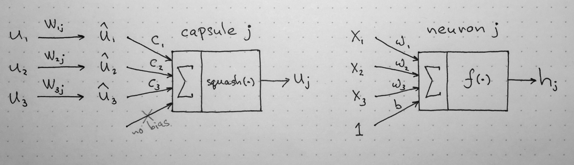
Left: capsule diagram; right: artificial neuron. Source: author, inspired by the talk on CapsNets given by naturomics.
On the other hand, the capsule has vector forms of the above 3 steps in addition to the new step, affine transform of input:
- matrix multiplication of input vectors
- scalar weighting of input vectors
- sum of weighted input vectors
- vector-to-vector nonlinearity
Let’s have a better look at the 4 computational steps happening inside the capsule.
1. Matrix Multiplication of Input Vectors
Input vectors that our capsule receives ($u_1$, $u_2$ and $u_3$ in the diagram) come from 3 other capsules in the layer below. Lengths of these vectors encode probabilities that lower-level capsules detected their corresponding objects and directions of the vectors encode some internal state of the detected objects. Let us assume that lower level capsules detect eyes, mouth and nose respectively and out capsule detects face.
These vectors then are multiplied by corresponding weight matrices $W$ that encode important spatial and other relationships between lower level features (eyes, mouth and nose) and higher level feature (face). For example, matrix $W_{2j}$ may encode relationship between nose and face: face is centered around its nose, its size is 10 times the size of the nose and its orientation in space corresponds to orientation of the nose, because they all lie on the same plane. Similar intuitions can be drawn for matrices $W_{1j}$ and $W_{3j}$. After multiplication by these matrices, what we get is the predicted position of the higher level feature. In other words, $\hat{u}_1$ represents where the face should be according to the detected position of the eyes, $\hat{u}_2$ represents where the face should be according to the detected position of the mouth and $\hat{u}_3$ represents where the face should be according to the detected position of the nose.
At this point your intuition should go as follows: if these 3 predictions of lower level features point at the same position and state of the face, then it must be a face there.
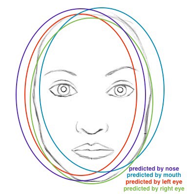
Predictions for face location of nose, mouth and eyes capsules closely match: there must be a face there. Source: author, based on original image.
2. Scalar Weighting of Input Vectors
At the first glance, this step seems very familiar to the one where artificial neuron weights its inputs before adding them up. In the neuron case, these weights are learned during backpropagation, but in the case of the capsule, they are determined using “dynamic routing”, which is a novel way to determine where each capsule’s output goes. I will dedicate a separate post to this algorithm and only offer some intuition here.
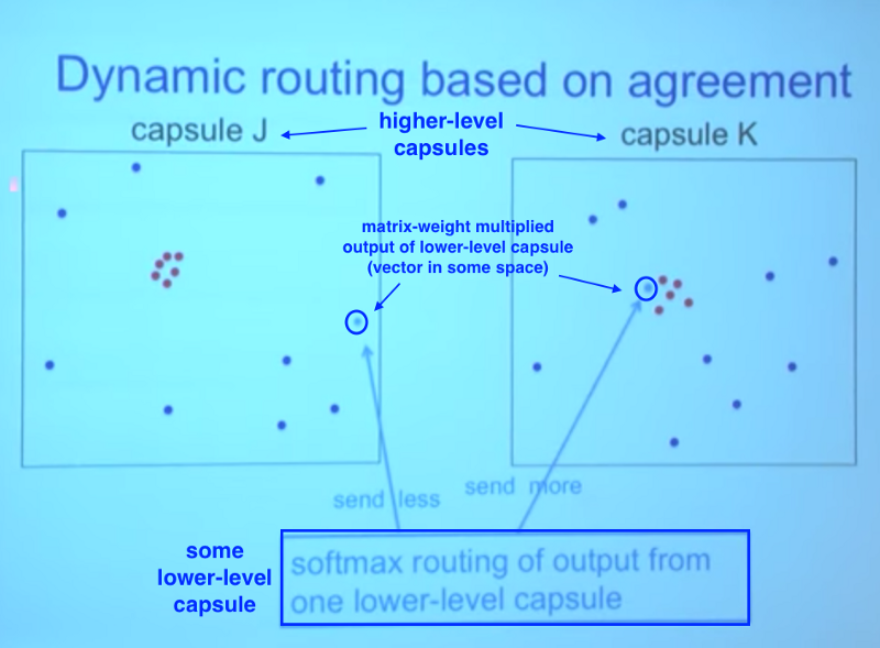
Lower level capsule will send its input to the higher level capsule that “agrees” with its input. This is the essence of the dynamic routing algorithm. Source.
In the image above, we have one lower level capsule that needs to “decide” to which higher level capsule it will send its output. It will make its decision by adjusting the weights $C$ that will multiply this capsule’s output before sending it to either left or right higher-level capsules $J$ and $K$.
Now, the higher level capsules already received many input vectors from other lower-level capsules. All these inputs are represented by red and blue points. Where these points cluster together, this means that predictions of lower level capsules are close to each other. This is why, for the sake of example, there is a cluster of red points in both capsules $J$ and $K$.
So, where should our lower-level capsule send its output: to capsule $J$ or to capsule $K$? The answer to this question is the essence of the dynamic routing algorithm. The output of the lower capsule, when multiplied by corresponding matrix $W$, lands far from the red cluster of “correct” predictions in capsule $J$. On the other hand, it will land very close to “true” predictions red cluster in the right capsule $K$. Lower level capsule has a mechanism of measuring which upper level capsule better accommodates its results and will automatically adjust its weight in such a way that weight $C$ corresponding to capsule $K$ will be high, and weight $C$ corresponding to capsule $J$ will be low.
3. Sum of Weighted Input Vectors
This step is similar to the regular artificial neuron and represents combination of inputs. I don’t think there is anything special about this step (except it is sum of vectors and not sum of scalars). We therefore can move on to the next step.
4. “Squash”: Novel Vector-to-Vector Nonlinearity
Another innovation that CapsNet introduce is the novel nonlinear activation function that takes a vector, and then “squashes” it to have length of no more than 1, but does not change its direction.
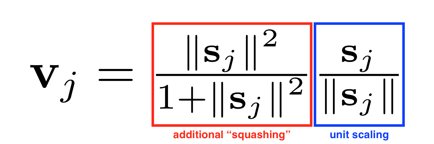
Squashing nonlinearity scales input vector without changing its direction.
The right side of equation (blue rectangle) scales the input vector so that it will have unit length and the left side (red rectangle) performs additional scaling. Remember that the output vector length can be interpreted as probability of a given feature being detected by the capsule.
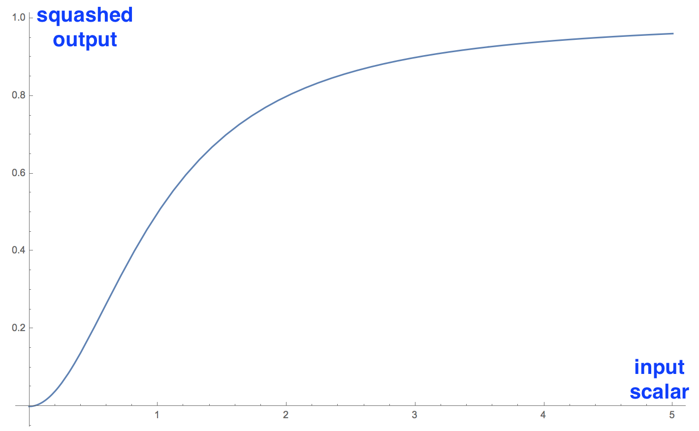
Graph of the novel nonlinearity in its scalar form. In real application the function operates on vectors. Source: author.
On the left is the squashing function applied to a 1D vector, which is a scalar. I included it to demonstrate the interesting nonlinear shape of the function.
It only makes sense to visualize one dimensional case; in real application it will take vector and output a vector, which would be hard to visualize.
Conclusion
In this part we talked about what the capsule is, what kind of computation it performs as well as intuition behind it. We see that the design of the capsule builds up upon the design of artificial neuron, but expands it to the vector form to allow for more powerful representational capabilities. It also introduces matrix weights to encode important hierarchical relationships between features of different layers. The result succeeds to achieve the goal of the designer: neuronal activity equivariance with respect to changes in inputs and invariance in probabilities of feature detection.
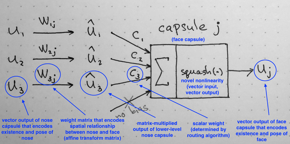
Summary of the internal workings of the capsule. Note that there is no bias because it is already included in the W matrix that can accommodate it and other, more complex transforms and relationships. Source: author.
The only parts that remain to conclude the series on the CapsNet are the dynamic routing between capsules algorithm as well as the detailed walkthrough of the architecture of this novel network. These will be discussed in the following posts.