ZFNet [2013, paper by Zeiler et al.]
Main ideas
Deconvolution, transfer learning (supervised pretraining is the term used in the paper), learning rate annealing with momentum
Why it is important
This architecture won the ImageNet competition in 2013, achieving the error rate of 14.8% (compared to 15.4% in the previous year).
Besides, this paper introduced a way to visualize learned convolutional features. Before this work, convolutional neural networks were pretty much black boxes, whose internal workings were unknown. This paper offered essential insights into how convolutional neural networks are learning internal representations. To achieve this goal, the authors introduce a way to map learned features into input pixel space by using a specially designed Deconvolutional Network.
Brief description
Deconvolution
Before I get into the application of deconvolutions in this paper, first I would like to note that you should not confuse deconvolutions in deep learning with deconvolutions in signal processing, they are very different. In deep learning, deconvolutions are also called transposed convolution and partially strided convolutions. Below, I explain why the term transposed is used.
Convolution allows going from a specified input dimension to some output dimension. Note that the shape of the output dimension is defined by parameters of a given convolution: input size, kernel size, strides, and padding. Deconvolution (transposed convolution) allows to go in the opposite direction: from the output dimension go back to the input dimension. Why would such operation be necessary? There are two reasons:
- deconvolution is used during backpropagation of error through the convolutional layer
- deconvolution is used for upscaling of input in specific deep learning applications such as superresolution and hourglass networks, to name a few.
Backpropagation for the convolutional layer is a deconvolution operation applied to the incoming gradient of the convolutional layer. If you look at convolution operation as the matrix multiplication of input by a convolution matrix $C$ (which is defined by the convolution kernel weights), then backpropagating the error is equivalent to multiplying the incoming gradient by the transpose of the convolution matrix $C$. This is why deconvolution is also called transposed convolution. Note that multiplying by the transposed convolution matrix, $C^T$, is equivalent to deconvolution with filters rotated by 180 degrees.
As for using deconvolutions in upscaling, you perform deconvolution but learn new filters, so that convolutional filters from preceding layers don’t need to be reused.
Deconvolution Network for Learned Features Visualizations
Visualizations produced are reconstructed patterns from an input image coming from the validation set that cause high activations in a given feature map.
To produce input images that result in maximum activations, a separate Deconvnet is attached to the output of each layer whose features we want to visualize. Each Deconvnet itself is a neural network whose input is activations of a particular layer, and the output is an image depicting pixels that are responsible for maximum activation of a convolutional kernel of our interest for a given convolutional layer. In the paper, Deconvnet is described as a sequence of transposed convolutions, de-pooling and a special modified ReLU. The sequence of operations is the reverse of the steps that were used in the original neural network to produce a particular layer’s output. For example, let’s imagine we are interested in visualizing conv3 layer of some neural net. The computation below is performed to get to the output of the layer conv3:
input image -> conv1 -> relu -> conv2 -> relu -> pool -> conv3
Deconvnet attached to the output, will perform operations in reverse:
de-conv3 -> de-pool -> relu* -> de-conv2 -> relu* -> de-conv1 -> output image
The output of the Deconvnet has the same dimensions as the input image in the convnet we are visualizing.
Note that de-conv stands for deconvolution, this operation is also sometimes called transposed convolution. It uses transposed convolutional kernels of the original network that we want to visualize.
De-pooling operation (de-pool) is expanding dimensionality of data by remembering the pooled positions in the forward pass of the network we want to visualize.
Modified ReLU (relu*) only passes forward positive activation, this is equivalent to backpropagating only positive gradients, which is different from backpropagating through a regular ReLU. This is why the authors call it modified.
The paper is not very clear about why all these steps are necessary. After some research, I found another way to look at the Deconvnet: it is just a modified backpropagation step of the original convnet we are visualizing. Let’s get back to the example from above:
input image -> conv1 -> relu -> conv2 -> relu -> pool -> conv3
Backward pass for this computation looks like this:
backprop conv3 -> backprop pool -> backprop conv2 -> backprop relu -> backprop conv1 -> gradients of the input image
Now, backprop through a convolutional layer is just a deconvolution with the kernel rotated by 180 degrees (transposed convolution), so we have backprop conv = de-conv. Backprop through pooling is the same as de-pool as defined in the paper. Lastly, instead of using standard backpropagation through ReLU, the authors use modified ReLU, that only passes the positive activations. So, the backprop step now looks like this:
de-conv3 -> de-pool -> relu* -> de-conv2 -> relu* -> de-conv1 -> output image
To conclude, the Deconvnet is a slightly modified backward pass through a convnet that you are trying to visualize whose output is an image that produces the maximum activation of a selected convolutional kernel for a selected convolutional layer. That image lets you understand what kind of feature this kernel learned to recognize.
Understanding Features Visualizations
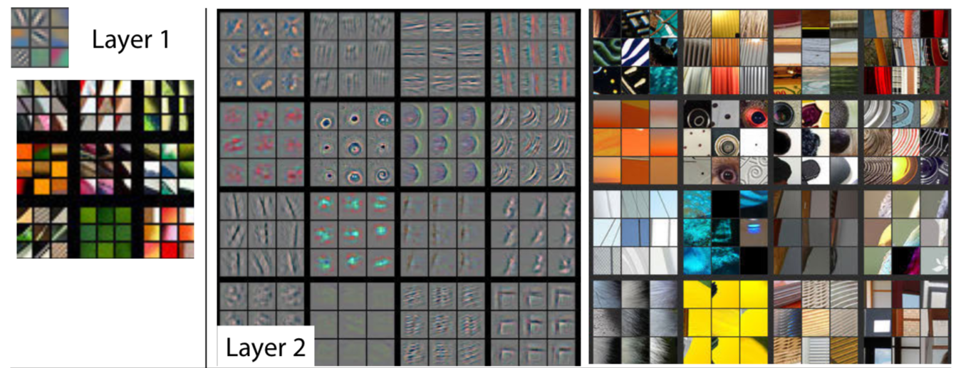
Examples of visualized features for layers 1 and 2. Note the size of activations projections and image patches are tiny for layer 1 and larger for layer 2. This has to do with different receptive fields of neurons in different layers. More on that below.
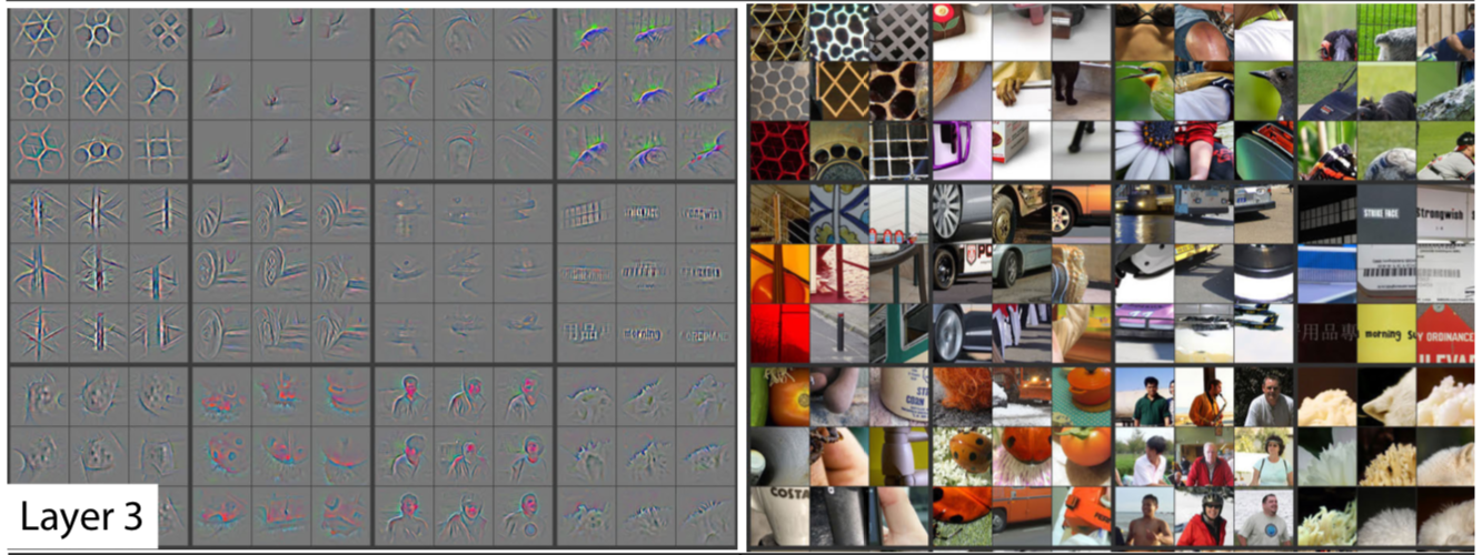
Examples of visualized features for layer3. Note the size of activations projections and image patches are somewhat small, but larger than in layers 1 and 2, and more complex.
The visualizations above are fascinating as they offer insights into the internal representation of knowledge learned by the network. It is essential to understand what precisely do they tell us. The images in the left side of the figures are projections from the highest activating neuron in a particular feature map to the pixel space of the input utilizing modified backpropagation outlined above. The images in the right side of the figure are parts of input images that produce a given projection on the left. In other words, visualization of activations is produced for each image separately.
Another critical thing to note is that the size of each of these projections is equal to each neuron’s receptive field upon the input image. Note that neurons in layers closer to the image have a smaller receptive field on the input image, and the further you go away from the image, the larger the receptive field becomes. I made a toy example in Excel that demonstrates that idea in figures below.
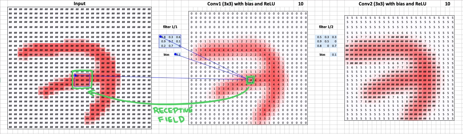
In this toy example, each neuron in the first convolutional layer looks at a 3 by 3 pixels patch of the input image.
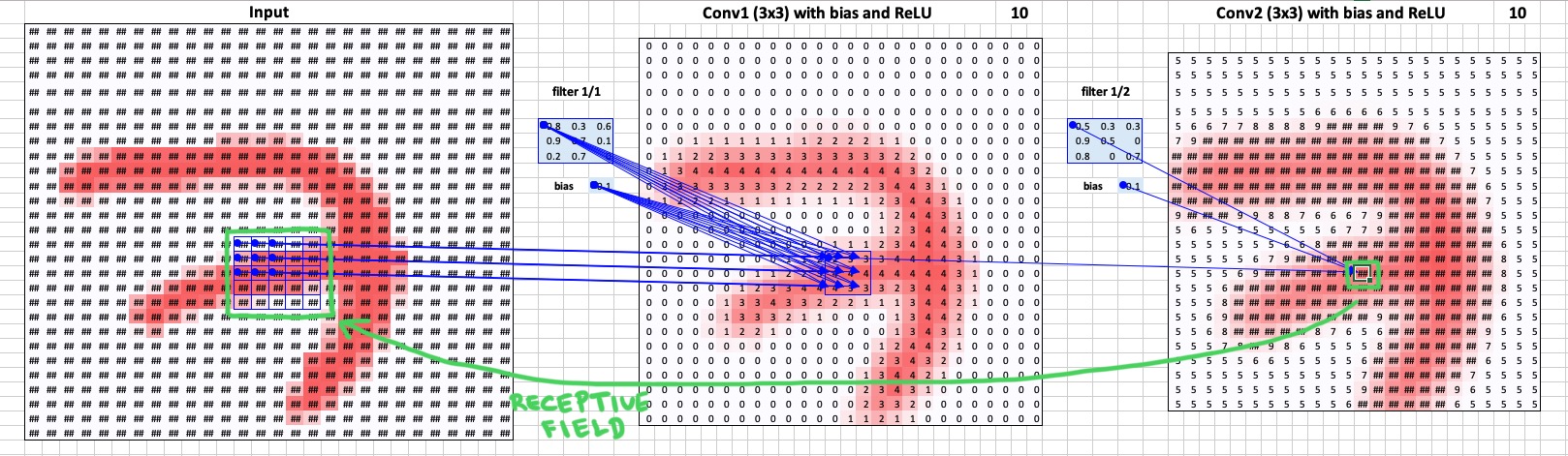
When you go to the next convolutional layer, each neuron looks look at a 5 by 5 pixels patch of the input image. Conclusion: the farther the layer is from the input, the larger the receptive field.
Now that you understand receptive fields recall that each convolution kernel slides across the input space and for each position it produces 1 activation. As a result, we have a 2D feature map for this kernel, consisting of numbers representing neuron activations. We can look and find the highest activation, and then we can trace back receptive fields through the network and find at which patch of the input image this particular highly activated neuron is looking. These patches are on the right side of the panel of each layer.
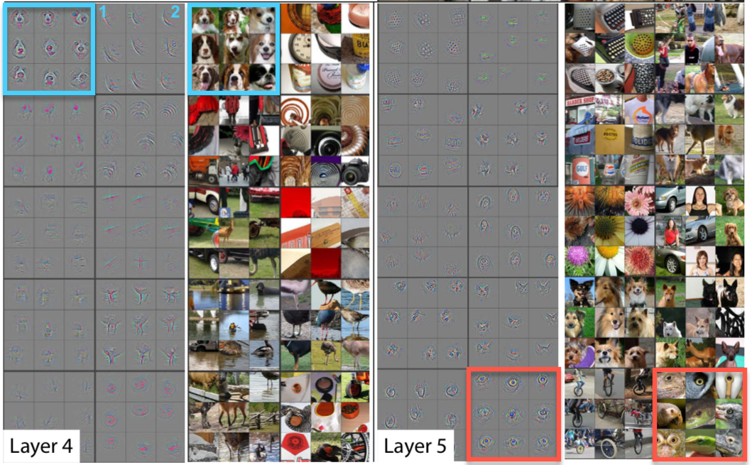
Examples of visualized features for layers 4 and 5. Note the size of activations projections and image patches are larger than those of layer 3. The complexity of detected entities is also higher than in previous layers.
Lastly, it is worth mentioning that the higher you go in the network (further away from the input), the more complex representations become. They increase complexity by combining more straightforward features from layers below. For example, if layer 2 detects circles, then layer 5 uses those detected circles when detecting god faces because dog eyes look like circles.
Architecture
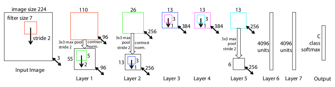
ZFNet architecture. Source: original paper.
Overall, the architecture of the network is an optimized version of the last year’s winner - AlexNet (you can read the detailed review here). The authors spent some time to find out the bottlenecks of AlexNet and removing them, achieving superior performance.
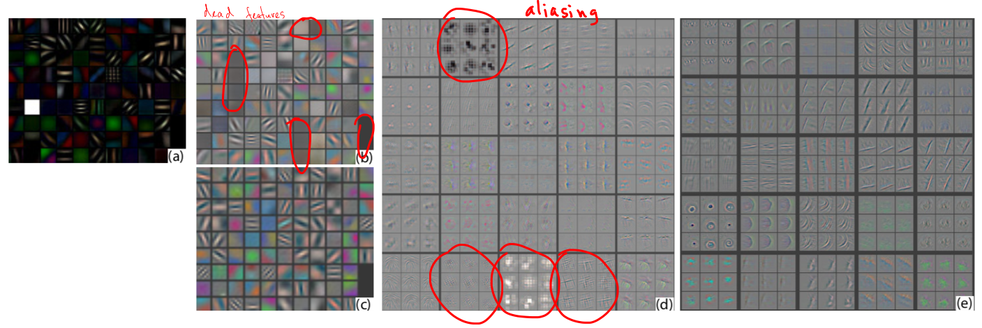
(a): 1st layer ZFNET features without feature scale clipping. (b): 1st layer features from AlexNet. Note that there are a lot of dead features - ones where the network did not learn any patterns. (c): 1st layer features for ZFNet. Note that are only a few dead features. (d): 2nd layer features from AlexNet. The grid-like patterns are so-called aliasing artifacts. They appear when receptive fields of convolutional neurons overlap and neighboring neurons learn similar structure. (e): 2nd layer features for ZFNet. Note that there are no aliasing artifacts. Source: original paper.
In particular, they reduced filter size in the first convolutional layer from 11x11 to 7x7, which resulted in fewer dead features learned in the first layer (see the image below for an example of that). A dead feature is a situation where a convolutional kernel fails to learn any significant representation. Visually it looks like a monotonic single-color image, where all the values are close to each other.
In addition to changing the filter size, the authors of FZNet have doubled the number of filters in all convolutional layers and the number of neurons in the fully connected layers as compared to the AlexNet. In the AlexNet, there were 48-128-192-192-128-2048-2048 kernels/neurons, and in the ZFNet all these doubled to 96-256-384-384-256-4096-4096. This modification allowed the network to increase the complexity of internal representations and as a result, decrease the error rate from 15.4% for last year’s winner, to 14.8% to become the winner in 2013.
To summarize, it was not a revolutionary change, but rather evolutionary, building upon the ideas of the previous year’s winner.
Additional readings
- Intuitively Understanding Convolutions for Deep Learning - pay attention to “Convolutions are still linear transforms” section, where a convolution is represented as a matrix-matrix multiplication (using so-called Toeplitz matrix)
- Stanford’s CS231n Winter 2017 Lecture 12
- A guide to convolutional arithmetic (with animations)
- Demystifying Convolution in Popular Deep Learning Framework — Caffe - low-level operations explained