Portfolio Project Report
Note: Code for this project can be found on my GitHub.
The goals / steps of this project are the following:
- Perform a Histogram of Oriented Gradients (HOG) feature extraction on a labeled training set of images and train a classifier Linear SVM classifier
- Apply a color transform and append binned color features, as well as histograms of color, to your HOG feature vector.
- Normalize features and randomize a selection for training and testing.
- Implement a sliding-window technique and use a trained classifier to search for vehicles in images.
- Run pipeline on a video stream and creating a heat map of recurring detections frame by frame to reject outliers and follow detected vehicles.
- Estimate a bounding box for vehicles detected.
0. Preface
Functionality-wise, all code for this project is stored in file utils2.py. I also make use of some functions from previous project, which is in file utils.py. All the processing steps and my project workflow, as well as some textual comments and visualization are in Jupyter Notebook vehicle-detection.ipynb that comes with submission.
Repository also contains folder figures/ that contain all relevant visualizations used in this project.
1. Histogram of Oriented Gradients (HOG)
1.1 Data Preparation and Exploration
Before going into feature selection, I decided to prepare the data and perform data exploration and visualization.
First, I read all the images from data folders and put all of them in a single np.array that had 4 dimensions and shape: n_imgs x img_height x img_width x n_channels. In addition, I created another np.array with labels, that only had one dimension and shape of n_imgs.
I then used pickle package to store them on disk to save time in the future and not read all images separately.
Code for this is contained in Section 1 of Jupyter notebook. The function used from utils2.py is make_data().
In the next section, I visualized some of the data and also calculated descriptive statistics. Below are visualizations of 36 cars images, randomly selected from the data set. Not that all images in the data set present photos of cars taken from behind or slightly from the side. There are no photos taken from the front. This is useful for our project, but might not be so good for generalization of the algorithm. What if we also want to detect cars from the front? We would need new data for that.
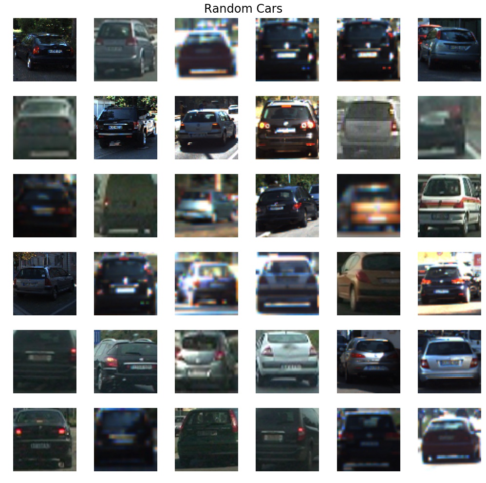
36 randomly selected car images from the data set.
And here are 36 non-cars images, randomly selected from the data set:
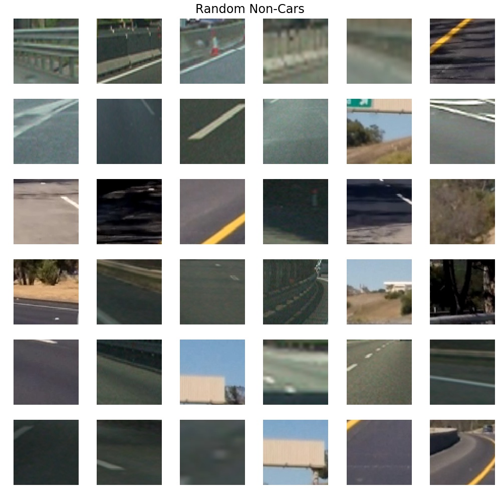
36 randomly selected non-car images from the data set.
To randomly select and plot data, I wrote a function plot_random_data().
I also paid attention to class sizes in order to make sure there is no class imbalance. There are 8792 cars in the data set and there are 8968 non-cars in the data set, which means data imbalance is not a problem and we should not worry about it.
I also played with different color channels to get a feel how they look. Function to do it interactively is in the notebook. It uses plotChannels() function in utils2.py.
1.2 Explain how (and identify where in your code) you extracted HOG features from the training images.
Feature extraction is performed in Section 3 of the notebook.
Most important functions that I used from utils2.py are extract_features() and summarize(). Extract features function is adapted from the classroom example.
As with many machine learning projects, there is no right answer to what features to use and what combination of parameters are the best ones. There are two approaches that I took to decide: reading other people’s results and playing with different values myself.
I saw that some other Udacity students only went with HOG features, and I decided to go with it at first. But when I got to video pipeline, I discovered that it did not work for me: false positives was a big problem and classifier was detecting cars where there definitely were no cars. I decided to fix this problem by expanding feature space with spatial features and color histogram feature. Not only did it help to reduce false positives occurrence, it also increased accuracy of classifier from 0.94 to more than 0.98, which is a quite substantial jump.
To summarize, there were 3 groups of features used to train classifier:
- HOG features (9 orientations, 8 pixels per cess, 2 cells per block, all hog channels for YUV color space)
- Spatial features (32 x 32 spacial dimension)
- Color histogram (32 bins in histogram)
1.3 Explain how you settled on your final choice of HOG parameters.
For HOG I tried different combinations and saw accuracy of classifier, eventually I stopped at said parameters. For spatial and color features, I used default values used in classroom and it worked at those values so I did not explore possibilities of fine-tuning those parameters.
Below I will show HOG images for car and non-cars for the same random subsample as figures above, they both are for R channel of RGB color space. It is only for visualization purpose to see some patterns. Even though I did not use RGB, it is still clear that cars and non-cars have different patterns of HOG edges. Cars have more complex patterns, whereas non-cars have a much simpler pattern comprising of one diagonal or a corner in most cases. Examples are below. There are similar visualizations at the end of this report for other channels.
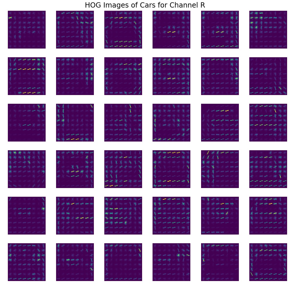
HOG features for the same 36 car images from above for the red color channel.
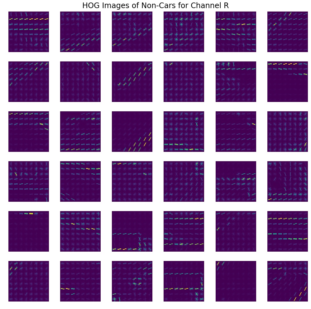
HOG features for the same 36 non-car images from above for the red color channel.
To produce HOG visualizations, I wrote a plot_hog_imgs() function that can be found in utils2.py.
1.4 Describe how (and identify where in your code) you trained a classifier using your selected HOG features (and color features if you used them).
After extracting the features and before training, I normalized the data to have zero mean and standard deviation of one. I used sklearn.preprocessing.StandardScaler for this purpose.
Here is the summary of data before normalization:

Statistics of non-normalized features.
And here is normalized data. Note that mean is very close to zero and SD is almost one.

Statistics of features after normalization. Note that mean is close to 0 and standard deviation is close to 1.
Then I needed to choose a classifier. At first I tried SVC but it took to long to train so I switched to LinearSVC. In addition to training faster, it only has one hyper-parameter: regularization coefficient C. I performed grid search over a range of value using GridSearchCV and determined that C of 0.001 was the best with reported accuracy of 0.9845 on the test set.
Accuracy is good, but what about false positive and false negative rates? To answer that I examined confusion matrices of this classifier, which can be seen below in both normalized and non-normalized flavors.
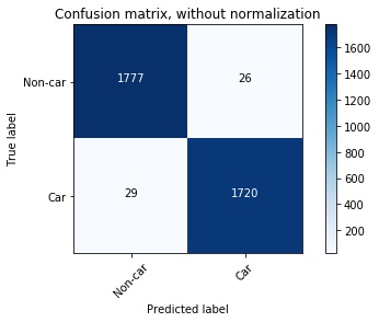
Confusion matrix for the trained classifier. Numbers in the boxes represent the number of training examples in each category.
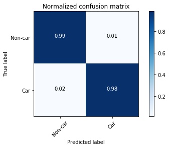
Confusion matrix for the trained classifier. Numbers in the boxes represent the proportion of training examples in each category.
1% false positive and 2% false negative rates are really good. This means that out of 3552 test images only 55 were misclassified. Not too bad. I pickled both classifier and scaler and proceeded to building detection system on images and then on videos.
To plot confusion matrices, I used plot_confusion_matrix() in utils2.py. I took it from sklearn documentation. Reference is in the comments of code.
2. Sliding Window Search
2.1 Describe how (and identify where in your code) you implemented a sliding window search. How did you decide what scales to search and how much to overlap windows?
In order to perform sliding window search, first a list of windows is generated and then algorithm tries to predict if there is a car in that window.
I developed a dynamically determined window size in the function box_size() in utils2.py. The idea is that objects that are farther away are smaller and therefore only need a small window to look for them. But how do we know if an object if far or close in the camera image? Well, the closer the object to the car, the closer it will be to the bottom of the image. And objects that are far from the car will be higher in the image. Therefore, it is possible to use vertical coordinate to determine an appropriate window size, which I did in the above mentioned function. It will take a vertical coordinate and return the size of the box corresponding to that coordinate. Below is and example, where higher windows have smaller size and lower windows have larger size.
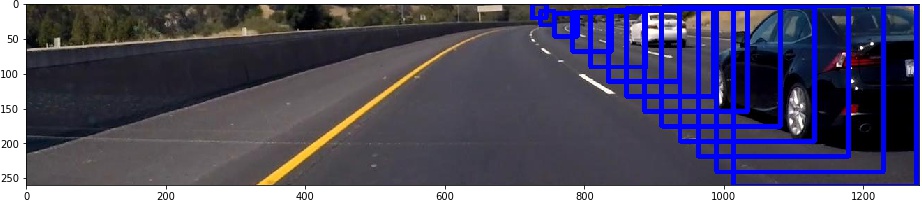
A sample of dynamically changing boxes. Closer cars are lower on the vertical axis and boxes are larger. Farther cars are higher on the vertical axis and boxes are smaller.
I had to play with parameters of that function to match sizes in such a way that car can be detected robustly.
Then I implemented function slide_dynamic_window() to generate windows to look in the image for cars. It will only look in the lower part of the image, because we are not interested in detecting cars where the sky is.
The function outputs a list of windows that can be applied to the image. I plotted a subset of those windows in the figure below.
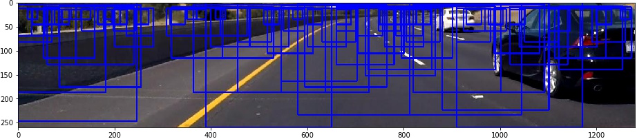
Random selection of sliding windows. I decided to only plot a selection because if I plotted all the boxes they would obscure the image itself.
The parameters used for sliding windows in the final pipeline were as follows:
- minimal size of 64 pixels
- maximal size of 160 pixels
- overlap of 50%
- size of the window determined by the vertical coordinate of the center of the window inside the image
2.2 Show some examples of test images to demonstrate how your pipeline is working. What did you do to optimize the performance of your classifier?
The pipeline works as follows:
- windows are generated
- each window is resized to 64 by 64 pixels
- HOG, spacial and color features are extracted, vector of length 4932 is produced
- feature vector is fed in the classifier and prediction is extracted
- windows with positive predictions are plotted to produce output as below (note a false positive in the left side of the image, we will deal with it by using thresholding and temporal accumulation of frames):
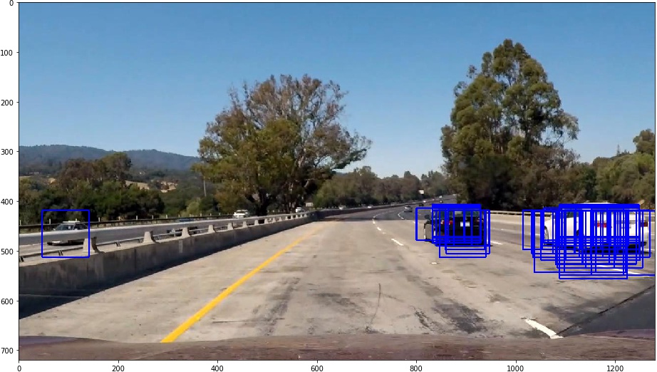
The main steps of a video frame processing pipeline.
To produce this result the following functions were implemented:
- box_size() to determine right size of candidate window
- draw_boxes() to draw detected boxes in the image
- slide_dynamic_window() to produce candidate windows
- search_windows() to return detected cars’ bounding boxes
3. Video Implementation
3.1 Simple Video Pipeline
To get rid of false positive and only have one bounding box per car, I followed approach offered by Udacity: heat maps with thresholding and labeling. The whole pipeline looks as follows:
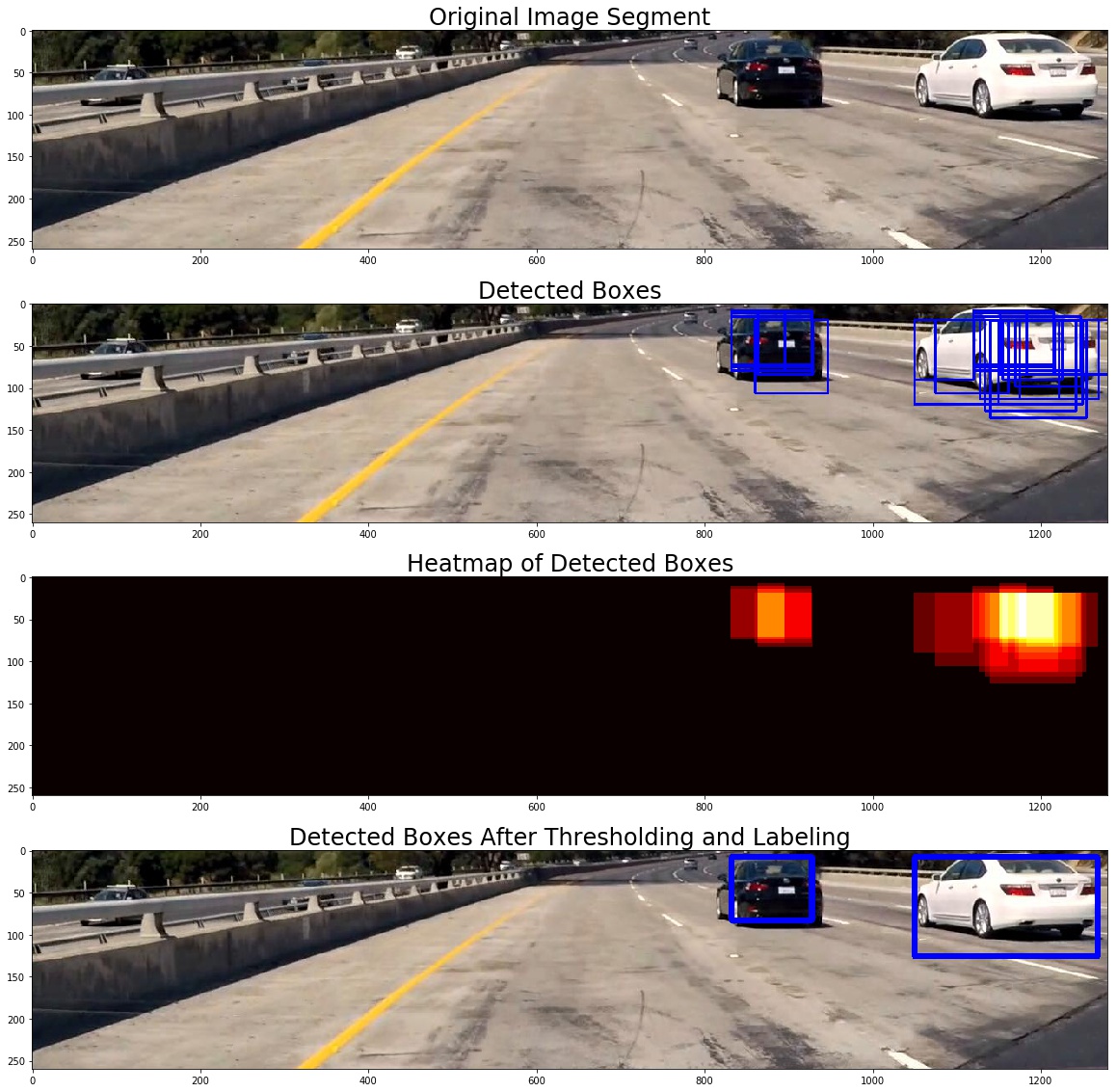
Caption
After receiving boxes for which classifier thinks that they are cars, we make a heat map of all the boxes, where each box contributes value of 1 for every pixel of that bounding box. For example, if for some pixel in the image, there are 5 intersecting bounding boxes, the value of corresponding pixel of the heat map will be 5.
Then we set to 0 all values below certain threshold and return the heat map. The value had to be set by trial and error.
Then we apply scipy.ndimage.measurements.label() to retrieve boxes of isolated regions of the heat map and these will be final bounding boxes that we draw on top of the image.
All these steps are implemented in function labeled_image() in utils2.py. It creates heat map, applies threshold, finds labels and draws them on the image. This function is the basis for the simple pipeline, that works on each frame individually and disregards whatever happens in frames before. The simple pipeline is implemented in function process_image_simple() in Section 5 of the notebook.
I will improve on it in section 3.2.
3.1 Provide a link to your final video output. Your pipeline should perform reasonably well on the entire project video (somewhat wobbly or unstable bounding boxes are ok as long as you are identifying the vehicles most of the time with minimal false positives.)
Final video for this project can be found at output_videos/final_video.mp4.
3.2 Describe how (and identify where in your code) you implemented some kind of filter for false positives and some method for combining overlapping bounding boxes.
After I implemented simple pipeline as described in section 3.1 of this report, there still were some of the false positives in the video. The fix was rather simple: I accumulated last 15 frames to calculate the heat map and then used thresholding and labeling as before to retrieve final bounding boxes. I had to play with the number of frames and value of threshold before I was satisfied, I stopped at 15 frames back and threshold value of 25. The pipeline is implemented in function process_image_advanced() in Section 6 of the notebook.
4. Discussion
4.1 Briefly discuss any problems / issues you faced in your implementation of this project. Where will your pipeline likely fail? What could you do to make it more robust?
As with any project there was a lot of trial and error. I tried different approaches and sometimes some of them did not work well. For example, in the beginning, I only used HOG features, but that resulted in too many false positives, so I had to incorporate spacial and color features in addition to HOG.
Not for the first time I see that hyper parameter tuning is one of the most important parts of any machine learning project. The challenge is that there are too many combinations and you do not know in advance which one is good and which one is bad. To deal with this, one needs to do experimentation and also learn from other practitioners.
I do not think that approach taken for vehicle detection in this project is particularly robust and a good way to go. First of all, it only recognizes cars from the back (because of data set). Secondly, it is hard to see how to generalize it well for other classes of objects, such as signs, pedestrians, traffic lights etc. I firmly believe that deep learning is the way to go, especially with such networks as Fast R-CNN that demonstrated amazing results and works really fast and really accurately.
This project uses heat maps accumulated over multiple frames. This means that if a car is moving very fast in the frame, it might get rejected by the algorithm. Another area where the algorithm might fail, is operating in dark conditions or when cars are positioned sideways toward the camera, because the classifier only learned to classify cars in daylight and from behind.
Even though I am confident that my algorithm is not very robust, this is not the point. I think the value of this project is not its production and real world readiness, but the learning that it helped me achieve. Now I feel more proficient in creating pipelines that use computer vision and machine learning techniques. In addition to that, I have a nice portfolio of projects to show to a potential employer.
P.S. This is the last project of the first term. It was a very difficult term and I did not expect it to be like that when I was starting. I am really happy that Udacity is bringing education in cutting edge technology at a very affordable price and provides materials that almost no universities teach at this point. I’d also like to thank all Udacity reviewers for providing valuable feedback and motivating me to keep learning, no matter how frustrating it can get from time to time.